Cynnwys
- Measuring statistical uncertainty for the admin-based population estimates
- Conceptual framework
- Caveats
- Clustering local authorities
- Fitting the Generalised Additive Model
- Uncertainty intervals
- Further work
- Annex A. Workflow summary for the calculation of the ABPE uncertainty intervals
- Annex B: List of local authorities by cluster
1. Measuring statistical uncertainty for the admin-based population estimates
We have been working in collaboration with Professor Peter Smith of the University of Southampton to develop measures of statistical uncertainty for Office for National Statistics (ONS) population estimates. "Uncertainty" refers to the quantification of doubt about the estimates. Uncertainty measures for the mid-year local authority population estimates were published in 2017. The methods are described in Methodology for measuring uncertainty in ONS local authority mid-year population estimates: 2012 to 2016.
The methodology uses a range of statistical bootstrapping techniques to create plausible simulated distributions for the population estimates. Bootstrapping is a method for assigning measures of accuracy to sample estimates (Efron and Tibshirani, 1993). Uncertainty intervals are taken from the simulated estimates.
We have built upon and further developed these methods to derive indicative uncertainty intervals for the experimental admin-based population estimates (ABPEs V3.0). We use a benchmark approach, comparing the ABPEs against the 2011 Census. Ultimately, the intention is that statistical uncertainty for the ABPEs will be derived through a Population Coverage Survey.
The ABPEs consist of estimates of the population size produced through linkage of administrative data, including Pay As You Earn (PAYE) and tax credits data, national benefits and Housing Benefit data, English and Welsh school census, Higher Education Statistics Agency (HESA), and data from the Patient Register (PR) and the Personal Demographics Service (PDS).
Methods for the production of the ABPEs are described in the Principles of ABPE V3.0 methodology.
Nôl i'r tabl cynnwys2. Conceptual framework
We use the following model:
where:
Pi,j,k is the true, unknown population size for local authority (LA), i=1, ... , 348, sex, j=1,2, and age, k=0, ... , 90
ABPEi,j,k is the ABPE estimate
LSFi,j,k is a log-scaling factor (LSF) – a measure of bias in the ABPE estimate
is the error.
By taking the exponential of both sides of this equation, the model can be written as:
We make the simplifying assumption that the error associated with the census is an order of magnitude smaller than the error associated with the ABPE, and therefore set it to zero. Thus:
To estimate the log-scaling factor LSFi,j,k, we compare the 2011 ABPE estimate, abpei,j,k, with the 2011 Census, denoted censusi,j,k, as an external benchmark representing the “true” population size.
Thus, we obtain the observed LSF:
When interpreting the LSFs, a value greater than zero indicates that fewer people have been captured by the ABPE than in the census data (ABPE undercount). Conversely, a value less than zero indicates that more people have been captured by the ABPE data than in the census data (ABPE overcount).
To create plausible simulated values for the LSFs, we need to estimate the error distribution, F. We make the assumption that the variability between LAs within a group of similar LAs is a good proxy for within-LA variability for the LAs within that cluster. We identify groups of similar local authorities through a cluster analysis of the LSF profiles by age and sex. The cluster analysis is run separately for males and females.
For each group of local authorities, a Generalised Additive Model (GAM) is fitted to the LSFs, generating predicted and residual values. The residuals are resampled to simulate an error distribution for each LA, by age and sex. This distribution of errors is added to the observed LSFs, and then back-transformed to generate a distribution of plausible population estimates. A step-by-step summary of the entire methodology is provided in Annex A.
Nôl i'r tabl cynnwys3. Caveats
Bear in mind the following caveats when considering these indicative uncertainty intervals:
These are interim measures of uncertainty, in place until the ABPE methodology is finalised.
This method does not allow for uncertainty in the 2011 Census estimates.
Nor does it allow for bias in the ABPEs to change as the intercensal decade progresses; instead, it assumes that bias observed with reference to the 2011 Census is propagated through the decade (further refinement may be possible once the ABPE methodology is finalised).
There is some circularity in this interim approach, since ABPEs have been tuned to 2011 Census estimates.
5. Fitting the Generalised Additive Model
Generalised Additive Models (GAMs) are fitted to the log-scaling factors (LSFs) by cluster. This semi-parametric approach was chosen because Rogers-Castro models that were used in mid-year estimate (MYE) uncertainty research were found to be a poor fit for LSF distributions, particularly for females. The GAMs generate fitted values denoted
and corresponding residuals, denoted ri,j,k. The clusters are denoted c=1, ... , 11, where clusters 1 to 5 correspond to females (four normal clusters and one for the outlier local authorities (LAs)) and 6 to 11 correspond to males (five normal, one outlier). An example of the data set following all the above processes is shown in Table 2.
For fitting the GAM, 22 knots are used for the age range of 0 to 90 years and over (one extra knot for ages 86 to 90 years, and an additional knot for age 90 years and over to account for the sharp difference in LSFs between ages 89 to 90 years and over). The knots are placed strategically to allow for more flexibility in the curve at minima and maxima. The knot locations were determined by:
- Starting with equally spaced knots (current best)
- Always keeping knots at age 0 to 90 years
- Randomly selecting 20 ages between 1 year and 89 years
- Fitting GAM
- Calculating a goodness of fit statistic (AIC)
- If the new AIC is better than the current best, then making this knot selection the current best
- Repeating 10,000 times (or as much as possible, given time constraints)
| Cluster | LA | Sex | Age | Census | ABPE | lsf | Fitted value | r |
|---|---|---|---|---|---|---|---|---|
| 3 | Amber Valley | F | 0 | 642 | 673 | -0.047 | -0.026 | -0.021 |
| Amber Valley | F | 1 | 631 | 650 | -0.030 | 0.024 | -0.054 | |
| …. | …. | …. | …. | …. | …. | …. | …. | |
| Amber Valley | F | 90 (+) | 816 | 790 | 0.032 | -0.014 | 0.046 | |
| ... | …. | …. | …. | …. | …. | …. | …. | …. |
| 4 | Wycombe | F | 0 | 1150 | 1161 | -0.010 | 0.013 | -0.022 |
| Wycombe | F | 1 | 1056 | 1046 | 0.010 | 0.025 | -0.015 | |
| …. | …. | …. | …. | …. | …. | …. | …. | |
| Wycombe | F | 90 (+) | 878 | 872 | 0.007 | 0.003 | 0.004 | |
| …. | …. | …. | …. | …. | …. | …. | …. |
Download this table Table 2: An overview of the data set following the clustering and GAM fitting processes.
.xls .csv6. Uncertainty intervals
We begin by defining a group as a unique combination of cluster, sex and age. For four normal clusters for females and five for males, plus one outlier cluster for each sex, there is a total of 11 clusters. Since there are 91 ages, there is a total of n = 11 x 91 = 1001 groups, each containing between 5 and 121 residuals (the number of local authorities (LAs) in the corresponding cluster).
We standardise the residuals so that the variance for each group is one, sample 1,000 residuals (with replacement) then reverse the standardisation. To standardise the residuals, denoted si,j,k, we divide each residual, ri,j,k, by its within-group standard deviation, σc,j,k, that is,
We calculate standardised residuals for each group in the “normal” clusters (1 to 4 and 6 to 10), creating 819 groups each with a variance of one. We assume that each group of standardised residuals follows the same underlying distribution1, and put them together in one pot (“Pot 1”).
The outlier clusters (5 and 11) are treated differently because of their unusual log-scaling factor (LSF) profiles. Instead of standardising their residuals, we assume the standard deviation is constant across all groups (within a cluster). Each group contains only five residuals, which is insufficient to obtain an accurate estimate of the standard deviation. Therefore, we allocate the raw residuals from cluster 5 to “Pot 2”, and from cluster 11 to “Pot 3”. The distributions of the residuals in each pot are shown in Figures 5a, 5b and 5c for LAs in the “normal” clusters, in the female outlier cluster and in the male outlier cluster, respectively.
Figure 5a: Distribution of the residuals in “Pot 1” (four “normal” clusters for females and five for males)
England and Wales, 2011
Source: Office for National Statistics
Download this chart Figure 5a: Distribution of the residuals in “Pot 1” (four “normal” clusters for females and five for males)
Image .csv .xls
Figure 5b: Distribution of the residuals for the female outlier cluster
England and Wales, 2011
Source: Office for National Statistics
Download this chart Figure 5b: Distribution of the residuals for the female outlier cluster
Image .csv .xls
Figure 5c: Distribution of the residuals for the male outlier cluster
England and Wales, 2011
Source: Office for National Statistics
Download this chart Figure 5c: Distribution of the residuals for the male outlier cluster
Image .csv .xlsFor each group in the normal clusters (1 to 4 and 6 to 10) 1,000 standardised residuals are resampled (with replacement) from Pot 1. The selected residuals are un-standardised by multiplying the selected residuals by the group standard deviation, σc,j,k.
For each group in clusters 5 and 11, 1,000 residuals are sampled (with replacement) from Pot 2 and 3, respectively. Since these residuals were not standardised, they do not need to be un-standardised.
Each set of 1,000 residuals is a simulated error distribution for all the LAs in the group, that is, it is an estimate of
in the first equation in Section 2. They are then added to the observed LSFs2, lsfi,j,k, to generate 1,000 simulated LSFs for each LA.
From the second equation in Section 2, the 1,000 simulated LSFs are back-transformed by exponentiating them to obtain 1,000 plausible scaling factors, and then multiplied by the published ABPE for LA i. Doing so, we obtain a simulated distribution of population estimates for each combination of sex, j, and age, k, within each LA, i.
The simulated distributions of population estimates are used to select an empirical 95% uncertainty for the true population size. The uncertainty interval is defined by the 2.5th and 97.5th percentile of the 1,000 simulated estimates.
Width of uncertainty intervals
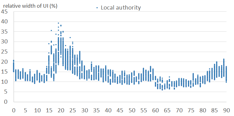
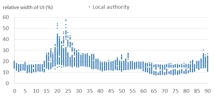
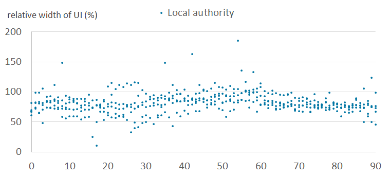
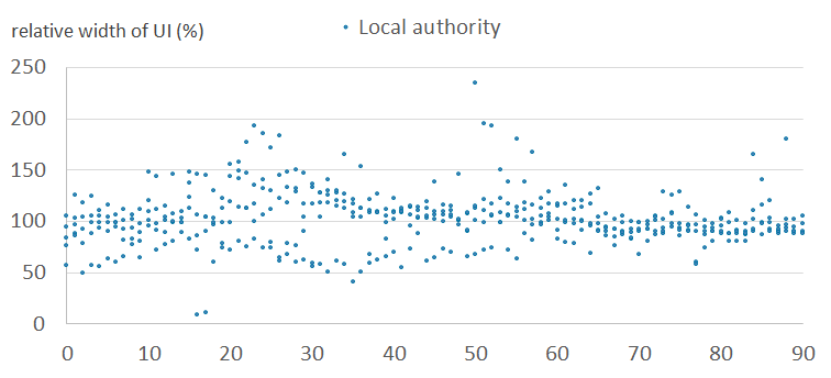
The relative width of an uncertainty interval (UI) is calculated as 100*(upper bound – lower bound)/ABPE. The larger uncertainty interval widths are a direct result of the larger group standard deviations.
Figures 6a and 6b show the relative width of uncertainty intervals by age for local authorities in the normal clusters, for females and males, respectively. Figures 6c and 6d show the equivalent results for local authorities in the outlier clusters. They show that the intervals are larger and more variable in the outlier clusters than in the normal clusters. This is because the outlier clusters contain local authorities whose scaling factor patterns vary greatly within cluster, and therefore the observed standard deviations are large. Uncertainty is typically higher for males than for females. Uncertainty varies by age, typically highest for student and young adult ages.
Figure 6a: Relative widths of the uncertainty intervals by age, for females - normal clusters (1 to 4)
England and Wales, 2011

Source: Office for National Statistics
Download this image Figure 6a: Relative widths of the uncertainty intervals by age, for females - normal clusters (1 to 4)
.png (35.9 kB)
Figure 6b: Relative widths of the uncertainty intervals by age, for males - normal clusters (6 to 10)
England and Wales, 2011

Source: Office for National Statistics
Download this image Figure 6b: Relative widths of the uncertainty intervals by age, for males - normal clusters (6 to 10)
.png (34.1 kB)
Figure 6c: Relative widths of the uncertainty intervals by age, for females - outlier cluster (5)
England and Wales, 2011

Source: Office for National Statistics
Download this image Figure 6c: Relative widths of the uncertainty intervals by age, for females - outlier cluster (5)
.png (15.4 kB)
Figure 6d: Relative widths of the uncertainty intervals by age, for males - outlier cluster (11)
England and Wales, 2011

Source: Office for National Statistics
Download this image Figure 6d: Relative widths of the uncertainty intervals by age, for males - outlier cluster (11)
.png (16.4 kB)Location of the ABPEs in their uncertainty intervals
We find that 15,689 (25%) ABPEs in the normal clusters and 69 (7.5%) in the outlier clusters lie outside their uncertainty interval (UI). This occurs when the middle 95% of the simulated scaling factors do not include 1. For them to contain 1, the corresponding simulated LSFs must contain 0 (log(1) = 0), and this can only happen if σ is large enough to extend the distribution sufficiently far out from the observed LSF. The census estimate always lies inside the uncertainty interval.
Figure 7a shows the distribution of the positions of the published ABPEs in their uncertainty intervals. The position is calculated as
where L is the lower bound of the uncertainty interval, and U is the upper bound. Therefore, a position of negative 1 means that the ABPE is the lower bound of the uncertainty interval, 0 means that the ABPE lies in the centre, and 1 means that the ABPE is the upper bound.
Figures 7b and 7c show how often the ABPEs fall outside of their uncertainty intervals for each age, by sex. The ABPEs fall outside most frequently for males aged 20 years, of working age, and from age 30 years to retirement, for both sexes.
Figure 7a: Distributions of the positions of the ABPEs within their uncertainty intervals, for all local authorities, ages and sexes
England and Wales, 2011
Source: Office for National Statistics
Notes:
- Four extreme values from clusters 5 and 11 are not shown in the histogram (5.29, 15.44, 16.10, 19.86).
Download this chart Figure 7a: Distributions of the positions of the ABPEs within their uncertainty intervals, for all local authorities, ages and sexes
Image .csv .xls
Figure 7b: The number of times the ABPE falls outside its uncertainty interval, by age for males
England and Wales, 2011
Source: Office for National Statistics
Download this chart Figure 7b: The number of times the ABPE falls outside its uncertainty interval, by age for males
Image .csv .xls
Figure 7c: The number of times the ABPE falls outside its uncertainty interval, by age for females
England and Wales, 2011
Source: Office for National Statistics
Download this chart Figure 7c: The number of times the ABPE falls outside its uncertainty interval, by age for females
Image .csv .xlsFigure 8 shows that for males aged 25 to 31 years, and 43 to 64 years in Richmondshire, the ABPE falls outside the 95% uncertainty interval.
Figure 8: ABPE, census and empirical 95% uncertainty intervals for males
Richmondshire, 2011
Source: Office for National Statistics
Download this chart Figure 8: ABPE, census and empirical 95% uncertainty intervals for males
Image .csv .xlsNotes for Uncertainty intervals
This assumption is supported by statistical testing of distributional differences using the two-sample Kolmogorov-Smirnof test, with Bonferroni correction for multiple comparisons.
The 1,000 resampled residuals are added to the observed LSFs as opposed to the fitted LSFs. This is because observed LSF values reflect relatively stable structural characteristics of LAs that are likely to persist over time.
7. Further work
The ABPE uncertainty intervals currently assume that bias in the ABPEs is unchanged as the decade following the census progresses. The inclusion of contemporaneous covariates would allow us to update the model, to account for change in the ABPE/Census relationship over time.
Explore the effects of clustering on the uncertainty intervals, including varying K (the pre-determined number of clusters), using hierarchical clustering, and choosing a subset of ages on which to base the clustering.
We also propose that further work could look at local authority-level analysis of the statistical uncertainty (as shown in Figure 8) and how it varies over time, place, and demographic group.
Nôl i'r tabl cynnwys8. Annex A. Workflow summary for the calculation of the ABPE uncertainty intervals
1. Import Census and ABPE estimates for each local authority (LA), i = 1, ... , 348 by sex, j = 1,2,and single year of age, k = 0, ... , 90(+).
2. Calculate the observed log-scaling factors (LSFs),
for all i,j,k
3. Identify unusual LAs separately for females and males based on the distance of their LSFs from the median LSFs and place them in two "outlier" clusters.
4. For each sex, cluster the remaining LAs based on similar patterns of LSFs across ages.
5. Fit a GAM to each cluster to obtain residuals, ri,j,k.
6. For each combination of “normal” cluster, sex and age (group), calculate the standard deviation of the residuals, σc,j,k.
7. For normal clusters, calculate the standardised residuals, si,j,k, by dividing each of the residuals, ri,j,k, by their group standard deviation, σc,j,k, i.e.
8. Put the standardised residuals into ”Pot 1”.
9. Resample 1,000 standardised residuals (with replacement) from Pot 1.
10. For each group in the normal clusters, un-standardise the selected residuals by multiplying the selected residuals by the group standard deviation, σc,j,k.
11. Put the raw residuals from the female outlier cluster into “Pot 2”, and those from the male outlier cluster into “Pot 3”.
12. For each group in the female (male) outlier cluster resample 1,000 residuals (with replacement) from Pot 2 (3).
13. For each group in all clusters, add the 1,000 residuals to the observed LSFs, lsfi,j,k, to generate 1,000 simulated LSFs for each LA.
14. To obtain a simulated distribution of population estimates for each LA by age and sex, exponentiate the 1,000 simulated LSFs (generating 1,000 plausible scaling factors), and then multiply each of them by the published ABPE.
15. For each LA by age and sex, use the simulated distribution of population estimates to calculate the uncertainty interval as follows: the lower and upper limits of the uncertainty intervals are the 2.5th and 97.5th percentile of the 1,000 simulated estimates.
Nôl i'r tabl cynnwys