Cynnwys
- Executive summary
- Introduction
- Small area estimation methods
- Construction of a linear mixed effects model for the FRS data
- Results
- Assessment against comparative estimates
- Concluding remarks and future work
- Acknowledgements
- References
- Appendix A: Fixed effects parameter estimates
- Appendix B: Random effects variance estimates
- Appendix C: Summary statistics for the MSOA percentile net weekly household income estimates
1. Executive summary
This report describes the application of the Empirical Best Predictor (EBP) method (Molina and Rao, 2010) to obtain estimates of the mean, median and other percentiles for household income for Middle Layer Super Output Areas (MSOAs) in England and Wales, using the 2011 household-level Census data and 2011 to 2012 Family Resources Survey (FRS) (Department for Work and Pensions, 2013). Estimates of distributions of household income are obtained for 2011.
We currently publish model-based estimates of the mean household income for MSOAs in England and Wales approximately every 3 years as a National Statistic. The mean has limitations as a measure of average income however, and users have said that they require more detailed distributions to make decisions about service provision and targeting resources.
The flexibility of the EBP method provides a potential solution since almost any measure of household income can be estimated under one methodology. This is because the EBP method predicts income for every household before aggregating them to the small area level. In the application described here robust estimates of household income are obtained for the 25th, 50th and 75th percentiles as well as the mean at the MSOA-level. The coefficient of variation (CV) for nearly all MSOA-level estimates was less than 0.20, and the average of the CVs for the mean household income was approximately 0.05. In other words, on average the variability of the mean household income estimates is small (5%) compared to the size of the estimate. The same was also true for the 25th, 50th and 75th percentiles.
Validation against alternative estimates, however, indicated that some caution should be used with the extremes of the distribution (10th and 90th percentiles). Nevertheless, the study illustrates how the use of one small area estimation method can assist us in meeting users’ requirements for more information on the household income distribution at more detailed geographies.
A limitation of the EBP approach is that household-level census data is required and so estimates can only currently be derived in census years. Work is currently being conducted to assess the options available for producing estimates in the non-census years. However, the EBP estimates could still be beneficial as an additional output to accompany the 2021 Census.
The EBP estimates of total household income at MSOA-level are benchmarked to regional total direct estimates from the FRS. This means that model-based EBP estimates of total income at MSOA-level, when aggregated at regional level, will match the corresponding direct estimates of total income obtained from the FRS survey data. There is currently no established solution for benchmarking nonlinear statistics such as percentiles. In this report, an intermediate solution is adopted.
Nôl i'r tabl cynnwys2. Introduction
2.1 Background
We currently produce model-based estimates of mean household income and of the proportion of households below the nationally defined poverty line for Middle Layer Super Output Areas (MSOAs) in England and Wales (ONS, 2010a; ONS, 2010b; ONS, 2015a). The model-based estimates of mean household income are published as National Statistics and are used by central government for policy development and monitoring, by local government for service planning and by private businesses to inform marketing strategies.
However, they have limitations in meeting user needs as the mean income provides little information about the distribution of income across households in an area and can be inflated by the relatively small number of households with very large incomes. Estimates of the median income are considered to be more useful because they are not affected by this skew in the income distribution. In addition, estimates of income for other percentiles would provide a more detailed description of income in an area and would better inform user requirements. For example, the income of the highest and lowest 25% of households would provide information on the disparity of income within an area.
The current method used by us for the estimates of mean income for small areas models data from the Family Resources Survey (FRS) (Department for Work and Pensions, 2013) in terms of area level aggregated variables and cannot be easily modified to estimate median income or other income quantiles. Advances in small area estimation, for example, the Empirical Best Predictor (EBP) method developed by Molina and Rao (2010), provides a flexible approach to estimating means, medians and percentiles of a specific study variable. The method relies on simulation techniques and uses estimates of the model parameters from a statistical model fitted to the FRS data to obtain estimates for the whole population. The simulated estimates are then used to derive summary measures for the distribution of interest. The EBP approach requires access to household-level census data in addition to the FRS data and is discussed in detail in Section 3.
The EBP approach also allows other measures that are a function of the household income to be computed by the process (for example, proportion of households in poverty in each small area). This is possible because the EBP method predicts each household income in each small area, before aggregating them to the small area level. This is a major advantage of this approach as it can produce several small area statistics under one unified methodology. Currently, we apply two separate methods to obtain mean household income and poverty statistics at MSOA-level.
This study, therefore, illustrates how the use of one small area estimation method can assist us in meeting users’ requirements for more information on the household income distribution at more detailed geographies.
2.2 Aims and extensions from the previous Empirical Best Predictor application
The Empirical Best Predictor (EBP) method has previously been evaluated at Office for National Statistics (ONS) using 2001 to 2002 FRS data and 2001 Census data for the North West and South East regions of England. In this initial research the natural logarithm of income (adjusted for household size and composition, after housing costs) was used as the response of interest for the statistical model fitted to the FRS data.
An outcome from this application was the concern with regards to the assumption of normally distributed errors for the fitted model at the household-level. If interest lies in estimating only the mean for each MSOA then it is well known that the fitted model is quite robust to deviations from this assumption. However, if interest lies in estimating the whole distribution of income for each MSOA, then the assumption of normally distributed errors becomes more crucial.
The objective of this next step in the research is the estimated household income distribution at MSOA-level for England and Wales by applying the EBP method to the 2011 to 2012 FRS data and 2011 Census data. Suitable transformations of the data to improve the fit of the model are also investigated. The study variable used in this application is the net weekly household income (adjusted for household size and composition, after housing costs). Results are shown for main summary measures of the household income distribution within MSOAs, namely: mean, median, and 10th, 25th, 75th and 90th percentiles. This study also considers all English regions and Wales as opposed to just the two English regions considered in the application using 2001 data.
A Box-Cox transformation of income is chosen as the best transformation of income for implementing the EBP approach (see Section 4 for more information) since it meets model assumptions better than the log transformation that was used in the previous ONS EBP application. In addition, in contrast to other alternative transformations considered, the Box-Cox transformation also avoids negative values when transforming back to the original income scale.
The EBP estimates are also adjusted to agree with direct survey estimates from the FRS of regional and country totals for England and Wales respectively (see Section 3 for more information). The EBP estimates are assessed by measuring their precision, comparing them against the current published model-based MSOA mean estimates as well as the direct estimates of mean income (based only on the FRS survey data) at regional level. Some external validation is also conducted by comparing the EBP estimates against direct estimates at local authority level from the Annual Survey of Hours and Earnings (ASHE).
This report is structured as follows. Section 3 introduces small area estimation methods and describes the current approach used by ONS to calculate the official MSOA model-based estimates of mean household income. It also describes the EBP approach developed by Molina and Rao to estimate means and percentiles for household income. The model fitted to the 2011 to 2012 FRS data with the Box-Cox transformation of income is discussed in Section 4. The results of the EBP application (point estimates and estimates of variability) for England and Wales are presented in Section 5. A detailed assessment of the quality of the EBP estimates is conducted in Section 6. Finally, the report concludes with a discussion of the results and recommendations for future work in Section 7.
Nôl i'r tabl cynnwys3. Small area estimation methods
3.1 Background
Small area estimation refers to techniques for combining survey, administrative and census data to improve the precision of direct (design-based) survey estimates. The techniques are employed when sample data are insufficient to provide direct estimates to an acceptable level of precision.
There are a number of methods; the more sophisticated of these work by taking advantage of various relationships in the data, drawing strength across sources, over space and time. They involve, implicit or explicit, statistical modelling to describe the relationships.
A common approach uses regression models to estimate the small area characteristics of interest and incorporates random area effects to account for between area variations beyond that explained by the model covariates (Fay and Herriot, 1979; Rao, 2003). The method depends on the availability of auxiliary information related to the variable of interest.
Once the relationship between the variable of interest and the auxiliary covariates have been established the estimated model coefficients can be used to obtain robust estimates for all small areas provided values are available for the explanatory covariates in the auxiliary data sources.
3.2 Approach currently in use for household income
In ONS, surveys are often designed to provide enough data for robust estimates for population characteristics at national or regional levels. However, estimates for smaller geographical areas such as for Middle Layer Super Output Areas (MSOAs) will be based on very few (or no) sample observations and are unlikely to provide accurate estimates. There are 7,201 MSOAs in England and Wales and each MSOA must have between 5,000 and 15,000 residents and between 2,000 and 6,000 households. Small area estimation is used to provide more accurate estimates for smaller geographical areas such as MSOAs.
Small area income estimates for England and Wales were first published by ONS in 2004 largely as a response to user demand for small area income data, which could not be met from the census. The current approach described in ONS (2010a), is to estimate the area (MSOA) level relationship between the survey variable (income) and auxiliary variables by regressing household responses from the Family Resources Survey (FRS) on MSOA values of the covariates. The auxiliary variables are generally average values of proportions relating to all individuals or households in the area and are based on administrative or census data with coverage in all the areas that are to be estimated. Once the model has been fitted the estimated model parameters are applied to the covariate values for each area to obtain the target estimates. While the model is constructed only on responses from sampled areas, the relationships identified are assumed to apply nationally.
The FRS is the survey with the largest sample that includes suitable questions on household income. Four survey variables are available for household income, providing options that account for household size, composition and housing costs. This detail allows valid comparisons of income between households to be made. The survey variables are:
total household weekly income
net household weekly income
net household weekly income (adjusted for household size and composition (equivalised)) before housing costs
net household weekly income (adjusted for household size and composition (equivalised)) after housing costs
The FRS aims to interview all adults in a selected household and has a response rate of approximately 62%. In 2011 to 2012 the FRS achieved a final sample size of 20,763 households in the UK and 15,541 for England and Wales. The current approach at ONS provides model-based estimates of mean household income at MSOA-level for all four types of income and for all 7,201 MSOAs in England and Wales. The natural logarithm of income was chosen as the response of interest for the fitted models to reduce the positive skew in the income distribution. It is assumed that the transformed variable follows a normal distribution. The model for income uses the following equation:
Equation 1
where yir is weekly income for household i in postcode sector (PCS)r
X̄k(ir) is the covariate population mean for MSOA k that household i in PCS r falls within; α and β are the regression parameters for the intercept and slope respectively; ur is the random error at PCS level assumed to have expectation 0 and variance σv2; and eir is the random error for household i in PCS r , with expectation 0 and variance σe2.
Only MSOA-level covariates are used for predicting income: for example, the proportion of people receiving benefits in the given MSOA. This gives an estimate of mean income across the area of interest. Estimates are currently produced at MSOA-level, with the area level random effect being defined at postcode sector (PCS) level.
The sampling area in the FRS is the PCS. As the FRS uses a clustered sample design, the area level variation in the model is measured using the PCS. It is assumed based on previous investigations that the variation for MSOAs is similar to variation for PCS however, and they are of similar size in terms of households. This means that the variance associated with the PCS can be used for error calculations relating to MSOAs. However, since there is no hierarchy between the PCS and MSOAs, the postcode sector random effect is ignored when it comes to obtaining the final estimates for MSOAs. An alternative approach is to model directly at MSOA-level with an MSOA-level random effect (see Section 3.3 for more information).
After modelling the estimates are benchmarked to the mean direct estimates of income from the FRS at region and country level for England and Wales respectively to ensure consistency between model-based and direct survey estimates.
Current methods employed by the ONS for producing model-based small area estimates of mean household income and the proportion of households in poverty require a separate modelling procedure. A household is defined to be in poverty if its income is below 60% of median income in the population. This is the definition for relative poverty used by the Organisation for Economic Co-operation and Development (OECD) and the European Union (Seymour, 2009). The model for the proportion of households in poverty has a binary response variable (1 if the household is in poverty and 0 otherwise). The model-based estimates of poverty are currently classified as Experimental Statistics and they were produced as a response to the desire for distributions on income.
Other desirable estimates, such as median household income, are not possible to obtain with the area based models currently employed by ONS because household- level estimates are required to calculate these.
3.3 Empirical Best Predictor (EBP) approach
A similar method to that used by the World Bank for poverty mapping is suggested by Molina and Rao (2010) and offers the possibility of a more flexible approach, which can be applied to obtain estimates for almost any percentile or measure required. The authors estimate nonlinear small area population parameters using the method and focus on estimating poverty indicators. In this application we adapt the method to estimate nonlinear small area parameters, focusing on household income.
The EBP method starts by fitting a standard mixed effects (multilevel) model, which relates the observed survey household income to a set of covariates common to both the survey and census (and distributed similarly in both). The estimated parameters of the distribution of the out-of-sample income can then be obtained using the estimated parameters from the fitted model.
The next step is to produce the EBP of the statistic we are interested in, for example, MSOA household median income, which will be the focus of this discussion. For each out-of-sample household in the population a fixed number of estimates of household income are simulated through random sampling of the estimated conditional distribution, and the median household income is found for each MSOA for each of these simulations. The EBP of median household income for an MSOA is then obtained by averaging over all of the medians obtained from each of the simulations for that MSOA. A full description of how the EBP estimates are obtained as well as how the method has been adapted for use in ONS are detailed in this section.
The final stage is to obtain an estimate of the variation associated with the estimated median. A parametric bootstrap sampling technique is applied, which samples from the distribution of the fitted model to produce a large number of bootstrap census populations where every household has an estimated income. The “true” median household income is obtained for each MSOA in each bootstrap population. From each bootstrap population a new FRS sample is drawn and the EBP estimation process applied to obtain a bootstrap estimate of the MSOA median household income. The mean square error (MSE) for each median can then be calculated from the “true” median household incomes and the estimated median household incomes.
Since estimates of income are obtained for individual households at each stage, it is relatively easy to obtain whatever small area statistic is required, for example, mean household income, median household income, and proportion of households in poverty. As mentioned in Section 2, the EBP approach also has the added advantage that all these statistics can be obtained under one framework rather than the existing approaches currently in use at ONS, which require separate modelling procedures for the mean household income and proportion of households in poverty.
In this application, the EBP method is used to produce estimates of household income at MSOA-level using the 2011 to 2012 FRS household-level covariates, household- and MSOA-level covariates sourced from the 2011 Census and MSOA covariates from the Department for Work and Pensions (DWP) administrative data. It is worth noting that the EBP approach uses covariates at both the household and MSOA-levels as opposed to the current approaches at ONS, which only use MSOA-level covariates.
Household-level covariates are vital for the EBP approach to give viable household-level predictions. The EBP method used in this application at ONS differs slightly from the traditional EBP approach described previously in that it was not possible to match the FRS sample households with the census households, which means that the observed incomes are discarded once the initial model is fit. As a consequence, incomes are simulated for all households in the population and not just the out-of-sample households.
As discussed in Section 3.2, the FRS has a clustered design based on the postcode sector (PCS) but this is ignored during the modelling process, with random effects defined at MSOA-level. This is deemed justifiable given that previous investigations found the variability at PCS level to be similar to the variability at MSOA-level. In addition, modelling at MSOA-level directly avoids the complications that would be encountered for the EBP approach with the PCS and MSOAs being non-nested geographies.
The method for obtaining the EBP estimates of the small area statistics for all MSOAs in England and Wales is outlined below. For illustration, MSOA median household income is used as an example of a statistic of interest and the Box-Cox transformation of income is used as the dependent variable for the fitted model. The EBP method involves the following steps.
Step 1: Multilevel model
A multilevel model is fitted to describe the relationship between the FRS income measurements and covariates sourced from the FRS, census and administrative sources. The census and administrative covariates used in the modelling process are at MSOA-level and the FRS variables are at the household-level.
The fitted model uses the following equation:
Equation 2
where Yik is the observed FRS income for household i in MSOA k, xik is a vector of the corresponding set of covariate values for household i in MSOA k (representing household- level and MSOA-level covariates), β is a vector of regression coefficients and c is the power that the income variable is raised to for the Box-Cox transformation. In addition, uk is the random effect for MSOA k, assumed to be normally distributed with expectation 0 and variance σu2, and eik is the within MSOA-level residual for household i in MSOA k, assumed to be normally distributed with expectation 0 and variance σe2. The random errors uk and eik are assumed to be independent.
Step 2: Simulate estimates of income
The next step is to produce a series of simulated estimates of income for each household in the census data and, subsequently, the required statistic for each MSOA in order to obtain the EBP for the small area estimate we are interested in. The income for household i that was not in the FRS sample in MSOA k, conditional on the sample data, is given by the following equation:
Equation 3
where εik are new errors and νk are new random effects. The εik are assumed to be normally distributed with expectation 0 and variance σe2. The νk are assumed to be normally distributed with expectation 0 and variance σu2 (1 - γk), with
γk = σu2 (σu2 + (σe2 / nk))-1, where nk is the sample size in MSOA k. The term μik is the ith element of the vector and is calculated using the following equation:
Equation 4
where Vks = σu2 1nk 1nk' + σe2 Ink, 1 denotes a vector of 1’s, Nk is the household population size for MSOA k, ks denotes the sample in MSOA k, and μk is evaluated for MSOA k.
To obtain a simulated estimate of income for each household within a small area (MSOA), we do the following:
a) an estimate of μk is calculated using Equation 4 and the estimates of the parameters β,σe2 and σu2 obtained from the model fitting in step 1
Remark 1: as we cannot identify which census households were sampled for the FRS, we apply Equation 4 to predict income for all households and not just out-of-sample households
b) a random sample of size Nk is drawn from N(0,σ̂e2 ), where Nk is the household population size for MSOA k; from this sample a value for εik is allocated to each household in the small area
c) a single random number is drawn from N(0, σ̂u2 (1 - γ̂k)); this will give a value for νk
d) a simulated income for each household i in MSOA k is then obtained from Equation 3 by using the census equivalent of the FRS covariate values xik with the estimated model coefficients β̂ and the values for μik, εik, and νk, obtained at a), b) and c), respectively – as for a), we apply the Equation 3 to all households and not just out-of-sample households; note that a back transformation is required to obtain the income estimates on the untransformed scale
e) the required small area estimate, for example, the median household income for the MSOA, is then calculated
Remark 2: step 2 assumes that all MSOAs are sampled in the FRS data. For MSOAs not sampled in the FRS, an adaptation of step 2 is needed. The household income is then predicted using Equation 2 with parameters replaced by their corresponding estimates obtained when fitting model (Equation 2) to the whole FRS data. Remarks 1 and 2 are applied when obtaining the results in Section 5.
Step 3: Repeat step 2
Step 2 is repeated for all MSOAs.
Step 4: Further repetition
Steps 2 and 3 are repeated a fixed number of times L (also known as Monte Carlo simulations). In the application reported in Section 5 , L is set equal to 50. We then have 50 estimates of median household income for each MSOA.
Step 5: Obtain the EBP
The Empirical Best Predictor of each MSOA median household income is then obtained by averaging the median household income across the 50 estimates in the MSOA.
Step 6: Bootstrap process
A bootstrap process is now applied to obtain the MSE of the estimates using random samples drawn from the fitted model (Equation 2) to generate bootstrap populations. This includes:
using the estimate of σe2 obtained from the fitted model (Equation 2), draw a random sample of size N from N(0,σ̂e2 ), where N is the population size; this gives a value for eir for each household in the population
using the estimate of σu2 obtained from the fitted model (Equation 2), draw a random sample of size R from N(0,σ̂u2 ), where R is the number of small areas; this gives a value for ur for each small area
with the random samples obtained previously, the estimated coefficients β̂, and the FRS covariate values replaced by the census equivalents, use the model (Equation 1) to generate a household income value for each household in the population; we now have one bootstrap population where every household has a household income value, which we take as the “true” income for this population and can calculate the ‘true’ median household income for each small area
select a new FRS sample from this bootstrap population and apply the Molina-Rao method outlined previously to obtain the EBP estimate for each area for this bootstrap population
repeat these steps B times, say B equals 250, to obtain 250 “true” median household incomes and 250 EBP estimates of median household income for each small area
The MSE for the small area estimate for area r is then found by using the following equation:
where Fr is the “true” median household income for small area r in bootstrap population b, Fr̂ is the estimate for small area r in bootstrap population b, and B is the total number of bootstrap populations generated.
Increasing the number of Monte Carlo samples will increase the accuracy of the estimates, and increasing bootstrap samples will increase the accuracy of the mean squared error estimates. Investigation demonstrated that increasing the number to 100 Monte Carlo samples and 500 bootstraps had relatively little impact on the quality of the results and doing so also increased the computational burden, particularly for the bootstrapping process.
3.4 Benchmarking
Most surveys based on probability sampling are designed to provide high quality statistics (unbiased, small variability) at national and regional levels and these are generally classified as National Statistics. Small area estimates derived from these same survey sources should be consistent with these estimates. For example, the official model-based estimates of mean household income at MSOA-level are benchmarked to the FRS national or regional level mean direct estimates.
The estimates from the previous application of the EBP approach were not benchmarked against direct estimates at national or regional level. The main reason for this is that there is no current established method for benchmarking nonlinear statistics such as percentiles. In this report, an intermediate solution is adopted. The EBP estimates of total household income at MSOA-level are benchmarked to national or regional total direct estimates from the FRS. This means that model-based EBP estimates of total income at MSOA-level, when aggregated at regional level, will match the corresponding direct estimates of total income obtained from the FRS survey data. Although this does not benchmark the percentiles of interest, it rescales the whole income distribution to reflect the new benchmarked total income. Since the adjustment is applied to all percentiles rather than just the centre of the distribution, the total is deemed more appropriate for this than the mean.
Nôl i'r tabl cynnwys4. Construction of a linear mixed effects model for the FRS data
In this section the methodology used to construct a predictive multilevel model for income is described. Note that while the current Office for National Statistics (ONS) estimates discussed in Section 3 include four types of income, this report focuses exclusively on net household weekly income after household costs and adjusted for household size and composition. This is one of the most commonly reported types of income.
The final sample size for the Family Resources Survey (FRS) in 2011 to 2012 was 15,541 households in England and Wales. However, the final analysis sample used in this application contains 15,162 households, after exclusion of 48 households with missing responses, 290 households with weekly incomes less than or equal to £1 (most of which were negative), 39 households with gross weekly incomes greater than £8,000 and 2 households were removed where the net weekly income was greater than the gross weekly income by £10 or more. Outlying values can have an unduly large influence on the fitted model. However, sensitivity analysis indicated that for this application removing the outlying observations of income did not make a notable difference to the estimated household income at an aggregate level.
A model that captures the relationship between a number of explanatory covariates and household income is required from the FRS data, which can then be used to predict income in the larger census dataset. This means that any variable included in the modelling of income at household-level needs to be in both the census and the FRS dataset (and distributed similarly in both); for variables not in the census and the FRS, only Middle Layer Super Output Area (MSOA) level covariates can be used. In addition, for categorical variables, the categories of the variables must perfectly match between the FRS and the census variables. In cases where the categories did not perfectly match, categories were collapsed accordingly if possible.
Section 4.1 discusses the covariates that were considered for inclusion in the fitted multilevel model. Section 4.2 focuses on model selection for the preferred transformation of income (Box-Cox transformation). Section 4.3 focuses on model diagnostics for the chosen multilevel model.
4.1 Choice of model covariates
The following household-level covariates (categorical unless otherwise specified), common to the 2011 to 2012 Family Resources Survey (FRS) survey and the 2011 Census, are considered in the model fitting:
Region of the household (forced in to the model)
Age group of household reference person
Gender of household reference person
Marital status of household reference person
Ethnic group of household reference person
Social classification of household reference person
Whether household reference person has ever worked
Whether anyone in household has long term illness
Number of adults in household (continuous variable)
Number of rooms in the household (continuous variable, maximum number of rooms is 10)
Household composition*
Household type of accommodation*
Household tenure*
Household density* (continuous variable, ratio of number of persons in the house to number of rooms)
Appendix A details the categories for the variables selected in the final multilevel model.
Notes:
*denotes a variable that was not considered in Small area estimates of income: means, medians and percentiles.
Age group of household reference person: This is available in the FRS as single year of age up until 79 years old but anyone aged 80 or over is classified as 80 years old. Therefore, age group was used rather than single year of age, which was used in Small area estimates of income: means, medians and percentiles.
Number of rooms is available in the FRS data but households with 10 rooms or more are classified as 10.
There were 24 households in the FRS data where the type of accommodation was missing. These were given the code for purpose-built flat or maisonette as most have one bedroom and with a tenure code for rents.
Highest qualification of household reference person was used in Small area estimates of income: means, medians and percentiles but in the 2011 to 2012 FRS data it is missing for 4,340 records (28.6%). This variable was not considered in this analysis.
The MSOA-level variables considered as potential covariates in this study (sourced from Census 2011 unless specified) refer to proportions of either households or individuals in an MSOA and are all logit transformed. These variables (untransformed) are as follows:
Proportion of households that are houses
Proportion of people aged 16 or less
Proportion of households in social group AB (highest two social grades combined)
Proportion of households that do not own a car
Proportion of people living in communal establishments
Proportion of people born in the UK
Proportion of households that contain a single person
Proportion of people aged 16 to 74 who are retired
Proportion of people aged 16 to 74 who are full-time students
Proportion of people who have a religion
Proportion of household residents living in a shared dwelling
Consumption of Ordinary Domestic Electricity as a proportion of total domestic energy consumption (sourced from the Department for Energy and Climate Change)
Proportion of people aged 16 and over claiming income support (sourced from the Department for Work and Pensions, forced in to the model)
It is advisable to reduce multicollinearity before any model selection procedures are conducted. A number of household-level and MSOA-level variables were not considered as potential covariates due to concerns over multicollinearity. For example, both number of rooms in the household and number of bedrooms in the household were not both included as potential household-level covariates due to multicollinearity. Only number of rooms in the household was included since this was deemed to be of more relevance. In addition, to avoid potential concerns over multicollinearity, no MSOA-level effect was allowed to be the same as a household-level effect. For example, whether the head of the household is employed and the proportion employed in an MSOA could not both be in the model.
4.2 Model selection for the Box-Cox transformation
To determine which of the covariates outlined in Section 4.1 should be retained in the multilevel model, the work presented in this report focused on a hierarchical selection approach. Firstly, stepwise selection procedures for the household-level covariates were conducted in the linear regression framework. The region of the household was forced in to the model before conducting any selection procedures. This is because the estimates produced using the Empirical Best Predictor (EBP) approach at Middle Layer Super Output Area (MSOA) level will be benchmarked to regional-level direct estimates of total income (equivalised after housing costs).
For any categorical variable where only some of the categories were found to be significant, the remaining categories were also included in the model. Covariates selected from this procedure were then added in to the multilevel model (MSOA treated as the random effect). Selection procedures were then conducted amongst the MSOA covariates using Akaike’s Information Criterion (AIC).
Due to the high number of categories in some variables, only interactions between binary and/or continuous variables were considered. Cross-level interactions and three-way interactions were not considered. The number of interactions included could not be too large otherwise the EBP process would fail to run due to the size of the matrices for the corresponding census covariates.
As discussed in Section 2, the Box-Cox (one parameter) transformation was applied for the fitted FRS model due to the fact it met model assumptions better than the logarithmic transformation of income that was used in the previous EBP report at ONS. This method uses the power family of transformations (see Draper and Smith, 1998, pages 279 to 281). A series of transformations of the form of Equation 5 are applied.
Equation 5
where Ẏ is the geometric mean of the response variable Y. Equation 5 is applied for a range of values for λ. A model is fitted for each of these versions of the transformed variable. Division by the geometric mean in Equation 5 standardises the log likelihood values so that these can be compared. The log likelihood for each model is plotted against λ. This will form a curve and the highest point of the curve is λ ̂, the maximum likelihood estimate of λ. This is the power to which the response should be raised to obtain the best fitting model. The method of course does not guarantee that the resulting model will be of an adequate fit.
Figure 1 shows the Box-Cox plot for the income variable. The value of λ was estimated to be 0.2 and the 95% confidence interval for λ did not include the value zero, which indicates that a log transformation is not recommended according to the Box-Cox method.
Figure 1: Box–Cox plot of log likelihood against lambda

Source: Office for National Statistics
Download this image Figure 1: Box–Cox plot of log likelihood against lambda
.png (12.2 kB)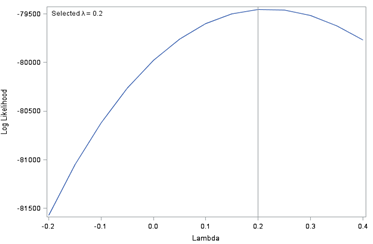
The hierarchical selection procedure described at the beginning of Section 4.2 was performed for the chosen Box-Cox transformation (income raised to the power 0.2). The parameter estimates for the selected multilevel model of the Box-Cox transformation are given in Appendices A and B. The q-q plot for the Box-Cox transformation is shown in Figure 2. Ideally the points will lie perfectly on the line y equals x in order for the normality assumption to be fully satisfied. Some improvements were gained compared to the log transformation but concerns remain with the extremes of the distribution. Further investigation by changing the power slightly from 0.2 for the Box-Cox transformation showed no improvement in the q-q plot. An advantage of the Box-Cox transformation compared to other potential transformations is that negative values cannot be encountered when transforming back to the original income scale.
Figure 2: Q-Q plot for income raised to the power 0.2

Source: Office for National Statistics
Download this image Figure 2: Q-Q plot for income raised to the power 0.2
.png (24.1 kB)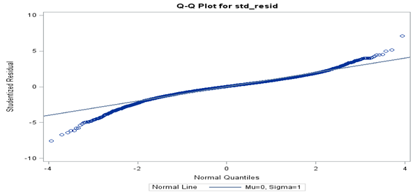
The FRS household-level covariates selected in the final multilevel model for the Box-Cox transformation are given in Table 1. These variables were present in both the FRS and the Census. Table 2 lists MSOA-level variables also selected in the final multilevel model.
Table 1: Variables included in both the 2011 to 2012 FRS data and the 2011 Census at household-level selected in the final model
| Variable |
|---|
| Region of the household (forced in to the model) |
| Age group of the household reference person |
| Gender of the household reference person |
| Ethnic group of household reference person |
| Social classification of the household reference person |
| Number of rooms in the household |
| Household density (log transformed) |
| Household composition |
| Household type of accommodation |
| Household tenure |
Download this table Table 1: Variables included in both the 2011 to 2012 FRS data and the 2011 Census at household-level selected in the final model
.xls (26.1 kB)
Table 2: Variables at MSOA-level from the census or Department for Work and Pensions datasets selected in the final model (all logit transformed and mean centred)
| Variable |
|---|
| Logit transform of the proportion of people in the social group ab |
| Logit transform of the proportion of households which do not own a car or van |
| Logit transform of the proportion of people aged 16 to 74 who are retired |
| Logit transform of the proportion of people aged 16 to 74 who are full time students |
| Logit transform of the proportion of people aged 16 and over who are on income support (forced in to model) |
Download this table Table 2: Variables at MSOA-level from the census or Department for Work and Pensions datasets selected in the final model (all logit transformed and mean centred)
.xls (26.1 kB)4.3 Model diagnostic for the Box-Cox transformation
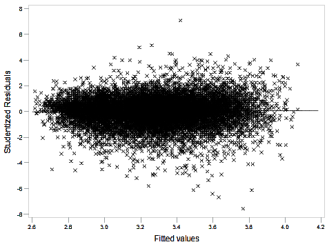
Normality of the household-level residuals was discussed in detail in Section 4.2. Further model diagnostics were examined to explore the validity of the multilevel model assumptions with the Box-Cox transformation (income raised to the power 0.2). Figure 3 plots the studentised residuals against the fitted values. The residuals are expected to fall in a random scatter with no obvious patterns. There is some evidence of increasing spread in the residual values as the fitted values increase, but it is not very extreme.
Figure 3: Studentised residuals plotted against the fitted values
Source: Office for National Statistics
Download this image Figure 3: Studentised residuals plotted against the fitted values
.png (39.1 kB)
The Cook’s distance measure was used to assess whether any observations (households) were having an undue effect on the parameter estimates. Values greater than one are often considered to be a cause for concern. No values were found to be greater than one.
Multicollinearity was reduced prior to conducting any selection procedures, as discussed in Section 4.1 . The normality of the MSOA random effects was assessed with no cause for concern found. The fitted model assumes that the covariates follow a linear relationship with the dependent variable. The variable household density was log transformed to avoid concerns over nonlinearity.
Appendices A and B provide the estimated coefficients and corresponding standard errors for the selected covariates in the model, including two-way interactions. Appendix B shows that the estimated variances at MSOA-level and household-level are 0.0011 and 0.1209, respectively. For a model with no fixed effects (null model), the variance estimates for the MSOA-level and household-level random effects are 0.0187 and 0.1686, respectively. This indicates that the full model accounts for 94% (100 multiplied by (1-0.0011 divided by 0.0187)) of the MSOA-level variability. The intraclass correlation for the chosen model is 0.9% (100 multiplied by 0.0011 divided by (0.0011 plus 0.1209)), indicating that a very small portion of the total variability is due to differences across MSOAs.
Note that this does not describe how much variation is explained by the fixed effects terms, which is more difficult to describe for linear mixed effects models. If the random effect at MSOA-level (uk) is removed from the model then the adjusted R squared is 0.35, which implies that there is still some variation unaccounted for by the model.
In Section 5, results for the household income distribution within MSOAs based on the Box-Cox transformation (income raised to the power 0.2) are presented.
Nôl i'r tabl cynnwys5. Results
The Empirical Best Predictor (EBP) method described in Section 3 is applied to estimate the household income distribution at Middle Layer Super Output Area (MSOA) level for all English regions (London, South East, South West, East of England, East Midlands, West Midlands, North East, North West, Yorkshire and The Humber) and Wales. The summary statistics estimated for each MSOA and reported in this section are the mean, median and 10th, 25th, 75th and 90th percentiles. These results are discussed in the following sections. The income variable considered is the net weekly household equivalised income after housing costs.
In addition, all results shown in this section have been benchmarked to regional total direct estimates from the Family Resources Survey (FRS) (see Section 3 for more information) and relate to the Box-Cox transformation of income (income raised to the power 0.2), which was found to be the most suitable transformation in terms of meeting model assumptions for the fitted FRS model. Results are given to the nearest British pound throughout the chapter.
The estimates are also accompanied by estimates of variability (coefficients of variation (CVs)). The CVs given are for the unbenchmarked estimates, as in Small area estimates of income: means, medians and percentiles. The reason for this is that the bootstrapping process used does not currently ensure that each simulated bootstrap population has regional totals that match the regional direct estimates from the FRS that were used for benchmarking in the point estimates process. The CVs for the unbenchmarked estimates are deemed to be a reasonable indication of variability.
5.1 Mean income
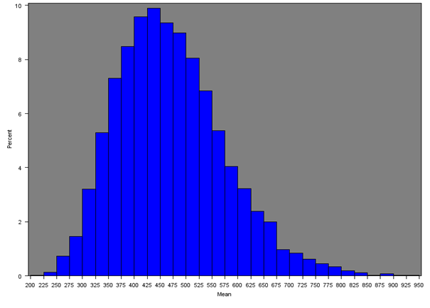
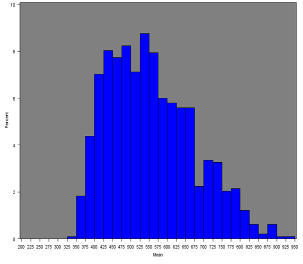
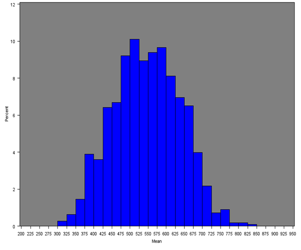
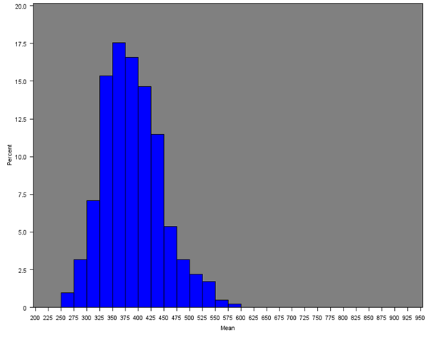
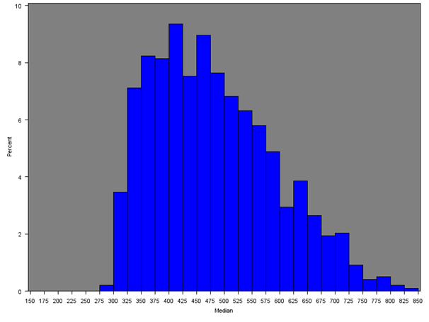
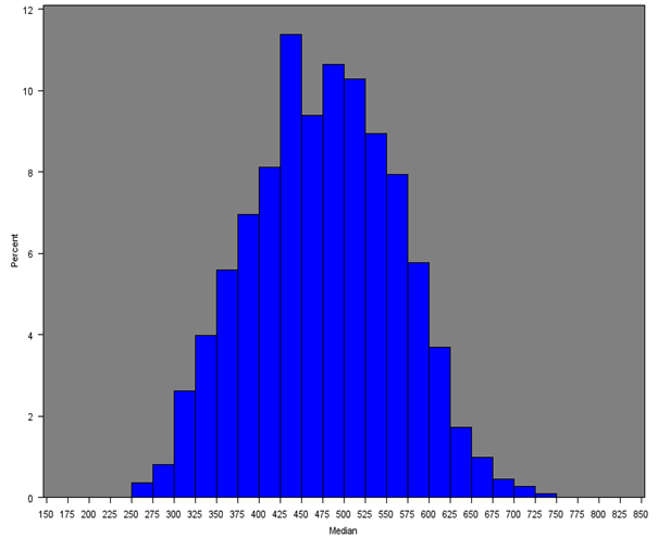
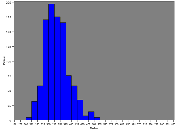
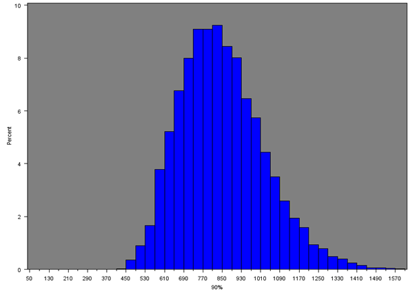
The mean weekly household equivalised income after household costs for each Middle Layer Super Output Area (MSOA) was calculated for all regions of England and Wales. Figure 4 shows the distribution of mean income across all MSOAs (England and Wales) and Figures 5a, 5b and 5c give the distribution of mean income across MSOAs for London, South East and Wales, which show notable distributions.
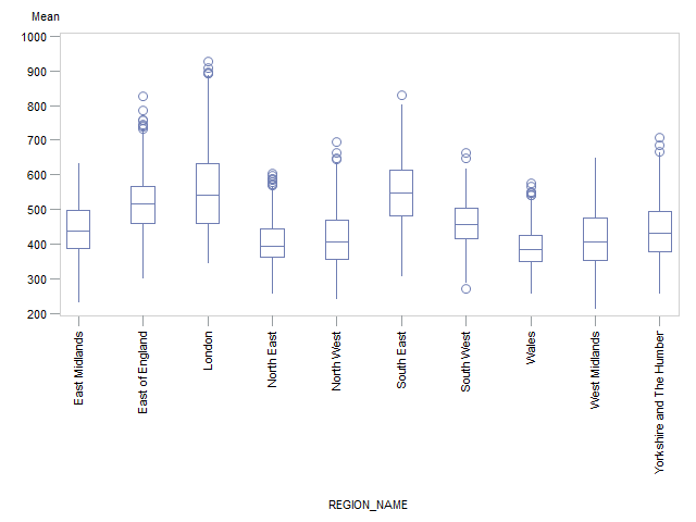
Figure 4 shows that the distribution across all MSOAs is skewed, with approximately 90% of MSOAs showing a mean weekly household income of approximately £300 to £650 per week, and less than 3% of MSOAs showing a very high weekly income of £700 per week or more. The median of the mean weekly income across all MSOAs is £460. Table 3 and Figure 6 show summary statistics and box-plots, respectively, for the mean incomes across English regions and Wales.
The South East distribution is more symmetrical with approximately 90% of MSOAs having a mean weekly income of approximately £400 to £700. The median of the mean weekly income in the South East is £547, which is higher than any other region. The second and third highest estimates were for London (£541) and the East of England (£514) respectively. London has a noticeably positively skewed distribution due to having more MSOAs with incomes over £700 than any other region (approximately 14%). Approximately 90% of MSOAs in London have a mean weekly income of £400 to £800.
Wales has a positively skewed distribution due to a small number of MSOAs with incomes over £500 (approximately 5%). The median of the mean weekly household income is £384 in Wales, which is lower than any other region.
Figure 4: Distribution of the mean net weekly household equivalised income after household costs for all MSOAs in England and Wales
Source: Office for National Statistics
Download this image Figure 4: Distribution of the mean net weekly household equivalised income after household costs for all MSOAs in England and Wales
.png (17.3 kB)
Figure 5a: Distribution of the mean net weekly household equivalised income after household costs for MSOAs in London
Source: Office for National Statistics
Download this image Figure 5a: Distribution of the mean net weekly household equivalised income after household costs for MSOAs in London
.png (19.9 kB)
Figure 5b: Distribution of the mean net weekly household equivalised income after household costs for MSOAs in the South East
Source: Office for National Statistics
Download this image Figure 5b: Distribution of the mean net weekly household equivalised income after household costs for MSOAs in the South East
.png (18.6 kB)
Figure 5c: Distribution of the mean net weekly household equivalised income after household costs for MSOAs in Wales
Source: Office for National Statistics
Download this image Figure 5c: Distribution of the mean net weekly household equivalised income after household costs for MSOAs in Wales
.png (17.8 kB)
Table 3: Summary statistics for the MSOA mean net weekly household income estimates, equivalised and after housing costs (EBP approach using Box-Cox income transformation) for English regions and Wales
| Region/Country | Number of MSOAs | Minimum (£) | 1st Quartile (£) | Median (£) | 3rd Quartile (£) | Maximum (£) |
|---|---|---|---|---|---|---|
| East Midlands | 573 | 235 | 389 | 439 | 496 | 634 |
| East of England | 736 | 303 | 458 | 514 | 567 | 828 |
| London | 983 | 346 | 461 | 541 | 632 | 926 |
| North East | 340 | 259 | 363 | 395 | 444 | 605 |
| North West | 924 | 243 | 355 | 408 | 470 | 696 |
| South East | 1108 | 310 | 481 | 547 | 613 | 830 |
| South West | 700 | 270 | 415 | 457 | 503 | 663 |
| West Midlands | 735 | 215 | 352 | 408 | 475 | 647 |
| Yorkshire and The Humber | 692 | 260 | 378 | 432 | 493 | 706 |
| Wales | 410 | 259 | 348 | 384 | 425 | 576 |
| All | 7201 | 215 | 395 | 460 | 534 | 926 |
| Source: Office for National Statistics | ||||||
Download this table Table 3: Summary statistics for the MSOA mean net weekly household income estimates, equivalised and after housing costs (EBP approach using Box-Cox income transformation) for English regions and Wales
.xls (27.6 kB)
Figure 6: Box-plot of the mean net weekly household equivalised income after household costs by region or country
Source: Office for National Statistics
Download this image Figure 6: Box-plot of the mean net weekly household equivalised income after household costs by region or country
.png (13.8 kB)
The distributions of the coefficients of variation (CV) are shown in Table 4 for each English region and Wales. These show that the estimates are accurate. The median CV for all regions is approximately 0.05 and the maximum CV is 0.196. Of the 7,201 MSOA mean estimates, a small number had CVs greater than 0.15 and there were no CVs over 0.20. In official statistics, estimates with CVs greater than 0.20 are typically considered less reliable.
Table 4: Coefficients of variation distribution for the MSOA mean household income estimates for each English region and Wales
| Region/Country | Number of MSOAs | Min CV | 1st Quartile | Median | 3rd Quartile | Max CV |
|---|---|---|---|---|---|---|
| East Midlands | 573 | 0.016 | 0.034 | 0.050 | 0.056 | 0.173 |
| East of England | 736 | 0.017 | 0.032 | 0.048 | 0.054 | 0.146 |
| London | 983 | 0.015 | 0.038 | 0.051 | 0.058 | 0.196 |
| North East | 340 | 0.020 | 0.039 | 0.051 | 0.058 | 0.136 |
| North West | 924 | 0.013 | 0.035 | 0.050 | 0.057 | 0.191 |
| South East | 1108 | 0.014 | 0.031 | 0.049 | 0.058 | 0.163 |
| South West | 700 | 0.016 | 0.034 | 0.049 | 0.055 | 0.157 |
| West Midlands | 735 | 0.017 | 0.035 | 0.050 | 0.056 | 0.179 |
| Yorkshire and The Humber | 692 | 0.017 | 0.032 | 0.050 | 0.057 | 0.144 |
| Wales | 410 | 0.019 | 0.032 | 0.050 | 0.056 | 0.174 |
| All | 7201 | 0.013 | 0.034 | 0.050 | 0.056 | 0.196 |
| Source: Office for National Statistics | ||||||
Download this table Table 4: Coefficients of variation distribution for the MSOA mean household income estimates for each English region and Wales
.xls (28.2 kB)5.2 Median income
The median household equivalised income after household costs was calculated for all English regions and Wales. Figure 7 gives the distribution of the median income across all MSOAs and Figures 8a, 8b and 8c give the distribution of median incomes for London, South East and Wales respectively.
Across all MSOAs, the median of the median MSOA weekly income is £398 as opposed to the median of the mean MSOA weekly income of £460 from Section 5.1. Only the South East (£477), London (£467) and East of England (£445) had estimates over £400; and only the North East and Wales had estimates less than £350.
Table 5 gives summary statistics for the median income by region or country. The histograms are similar to those for the mean income (both overall and for each region separately), with median MSOA weekly household income being lower than the mean due to the positive skew in the distribution of income.
Figure 7: Distribution of the median net weekly household equivalised income after household costs for all MSOAs

Source: Office for National Statistics
Download this image Figure 7: Distribution of the median net weekly household equivalised income after household costs for all MSOAs
.png (16.5 kB)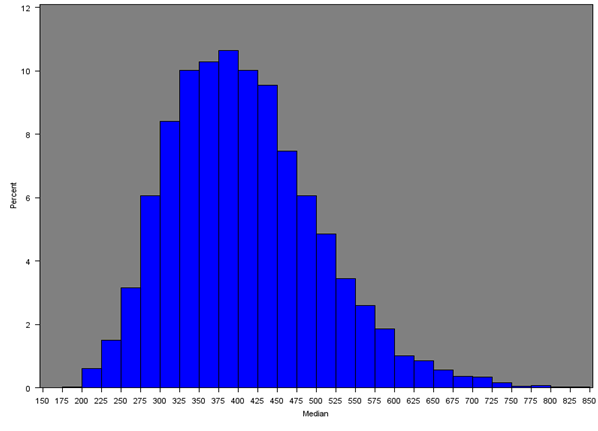
Figure 8a: Distribution of the median net weekly household equivalised income after household costs by region or country (London)
Source: Office for National Statistics
Download this image Figure 8a: Distribution of the median net weekly household equivalised income after household costs by region or country (London)
.png (17.4 kB)
Figure 8b: Distribution of the median net weekly household equivalised income after household costs by region or country (South East)
Source: Office for National Statistics
Download this image Figure 8b: Distribution of the median net weekly household equivalised income after household costs by region or country (South East)
.png (18.4 kB)
Figure 8c: Distribution of the median net weekly household equivalised income after household costs by region or country (Wales)
Source: Office for National Statistics
Download this image Figure 8c: Distribution of the median net weekly household equivalised income after household costs by region or country (Wales)
.png (16.9 kB)
Table 5: Summary statistics for the MSOA median net weekly household income estimates, equivalised and after housing costs (EBP approach using Box-Cox income transformation)
| Region/Country | Number of MSOAs | Minimum (£) | 1st Quartile (£) | Median (£) | 3rd Quartile (£) | Maximum (£) |
|---|---|---|---|---|---|---|
| East Midlands | 573 | 196 | 333 | 379 | 431 | 566 |
| East of England | 736 | 253 | 396 | 445 | 496 | 743 |
| London | 983 | 292 | 392 | 467 | 553 | 826 |
| North East | 340 | 217 | 310 | 340 | 387 | 536 |
| North West | 924 | 202 | 305 | 353 | 410 | 627 |
| South East | 1108 | 259 | 415 | 477 | 538 | 741 |
| South West | 700 | 224 | 357 | 395 | 437 | 595 |
| West Midlands | 735 | 177 | 301 | 352 | 412 | 573 |
| Yorkshire and The Humber | 692 | 218 | 323 | 374 | 428 | 635 |
| Wales | 410 | 217 | 298 | 330 | 368 | 513 |
| All | 7201 | 177 | 339 | 398 | 466 | 826 |
| Source: Office for National Statistics | ||||||
Download this table Table 5: Summary statistics for the MSOA median net weekly household income estimates, equivalised and after housing costs (EBP approach using Box-Cox income transformation)
.xls (27.1 kB)The distributions of the coefficients of variation (CV) are shown in Table 6 for each English region and Wales. These show that the estimates are accurate. The median CV for all regions is approximately 0.05 (to two decimal places) and the maximum CV is 0.203. Of the 7,201 MSOA median estimates, only two MSOAs had CVs over 0.20.
Table 6: Coefficients of variation distribution for the MSOA median household income estimates for each English region and Wales
| Region/Country | Number of MSOAs | Min CV | 1st Quartile | Median | 3rd Quartile | Max CV |
|---|---|---|---|---|---|---|
| East Midlands | 573 | 0.018 | 0.038 | 0.053 | 0.061 | 0.161 |
| East of England | 736 | 0.016 | 0.034 | 0.051 | 0.058 | 0.156 |
| London | 983 | 0.016 | 0.040 | 0.054 | 0.063 | 0.200 |
| North East | 340 | 0.021 | 0.040 | 0.055 | 0.063 | 0.149 |
| North West | 924 | 0.012 | 0.037 | 0.052 | 0.061 | 0.203 |
| South East | 1108 | 0.013 | 0.033 | 0.052 | 0.061 | 0.166 |
| South West | 700 | 0.017 | 0.036 | 0.052 | 0.059 | 0.167 |
| West Midlands | 735 | 0.017 | 0.039 | 0.053 | 0.061 | 0.187 |
| Yorkshire and The Humber | 692 | 0.017 | 0.036 | 0.053 | 0.061 | 0.169 |
| Wales | 410 | 0.020 | 0.034 | 0.053 | 0.059 | 0.172 |
| All | 7201 | 0.012 | 0.036 | 0.053 | 0.061 | 0.203 |
| Source: Office for National Statistics | ||||||
Download this table Table 6: Coefficients of variation distribution for the MSOA median household income estimates for each English region and Wales
.xls (28.2 kB)5.3 Income distribution
The Empirical Best Predictor (EBP) method can provide estimates for any percentile of interest although the extremes of the distribution can be estimated less precisely. Although the Box-Cox transformation used for the fitted model in Section 4 meets the normality assumption well, there are some concerns with the extremes of the distribution (see Figure 2).
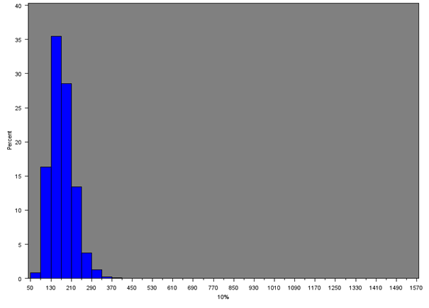
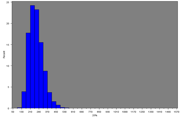
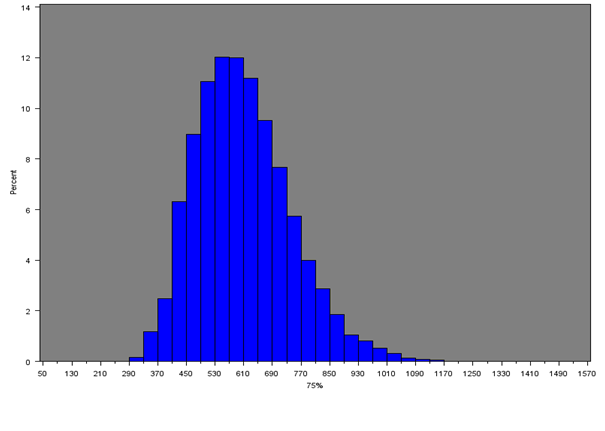
Figures 9a, 9b, 9c, 9d and 9e give the distribution of income for five percentiles (10th, 25th, 50th, 75th and 90th respectively ) across all MSOAs in England and Wales.
Table 7 shows summary statistics for each percentile of income across all MSOAs. Estimates in the extremes of the distribution (10th and 90th percentile) should be treated with more caution.
The median of the 25th percentiles of income across all MSOAs is £257 per week; so on average the bottom 25% of households within MSOAs have a weekly household income of £257 or less per week. Conversely, on average the top 25% of households within MSOAs have a weekly household income of £596 or more per week.
The lowest and highest 10% of the income distribution are of interest for determining areas that suffer from notable deprivation or wealth, respectively. Across all MSOAs, the median income for the 10th percentile is £167, whereas the median income for the 90th percentile is £832.
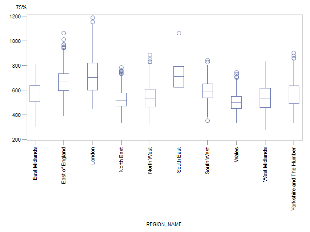
To give further insights into the disparity of income, Figures 10 and 11 show box plots by region or country for the distribution of the 25th percentile and 75th percentiles, respectively. Figure 10 shows that the median income across MSOAs for the 25th percentile is greatest in the South East (£310), London (£299) and East of England (£288) and lowest in the North East (£217) and Wales (£210).
London again has a noticeably positively skewed distribution and a wide range whereas the South East and East of England have a more symmetrical distribution and a smaller range. The North East and Wales both have a narrower range of values but the distribution in the North East is positively skewed whereas the distribution in Wales is more symmetrical. The same general conclusions were found for the 75th percentile (Figure 11). More detailed tables of results for the percentiles can be found in Appendix C.
Figure 9a: Distribution of 10th percentile of net weekly household equivalised income after household costs for all MSOAs
Source: Office for National Statistics
Download this image Figure 9a: Distribution of 10th percentile of net weekly household equivalised income after household costs for all MSOAs
.png (12.6 kB)
Figure 9b: Distribution of 25th percentile of net weekly household equivalised income after household costs for all MSOAs
Source: Office for National Statistics
Download this image Figure 9b: Distribution of 25th percentile of net weekly household equivalised income after household costs for all MSOAs
.png (12.6 kB)
Figure 9c: Distribution of 50th percentile of net weekly household equivalised income after household costs for all MSOAs

Source: Office for National Statistics
Download this image Figure 9c: Distribution of 50th percentile of net weekly household equivalised income after household costs for all MSOAs
.png (14.7 kB)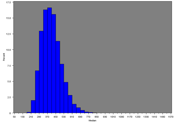
Figure 9d: Distribution of 75th percentile of net weekly household equivalised income after household costs for all MSOAs
Source: Office for National Statistics
Download this image Figure 9d: Distribution of 75th percentile of net weekly household equivalised income after household costs for all MSOAs
.png (14.3 kB)
Figure 9e: Distribution of 90th percentile of net weekly household equivalised income after household costs for all MSOAs
Source: Office for National Statistics
Download this image Figure 9e: Distribution of 90th percentile of net weekly household equivalised income after household costs for all MSOAs
.png (15.7 kB)
Table 7: Summary statistics of the MSOA percentiles for the net weekly household income estimates, equivalised and after housing costs (EBP approach using Box-Cox income transformation), England and Wales
| Percentile | Minimum | Median | Maximum | |
|---|---|---|---|---|
| (£) | (£) | (£) | ||
| 10th | 67 | 167 | 392 | |
| 25th | 108 | 257 | 563 | |
| 50th | 177 | 398 | 826 | |
| 75th | 279 | 596 | 1186 | |
| 90th | 410 | 832 | 1604 | |
| Source: Office for National Statistics | ||||
Download this table Table 7: Summary statistics of the MSOA percentiles for the net weekly household income estimates, equivalised and after housing costs (EBP approach using Box-Cox income transformation), England and Wales
.xls (26.6 kB)
Figure 10: Box plots by region or country for the 25th percentile of weekly household equivalised income after housing costs

Source: Office for National Statistics
Download this image Figure 10: Box plots by region or country for the 25th percentile of weekly household equivalised income after housing costs
.png (13.8 kB)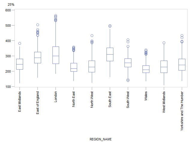
Figure 11: Box plots by region or country for the 75th percentile of weekly household equivalised income after housing costs
Source: Office for National Statistics
Download this image Figure 11: Box plots by region or country for the 75th percentile of weekly household equivalised income after housing costs
.png (13.2 kB)
Tables 8, 9, 10 and 11 show the distribution of the CVs for the 10th, 25th, 75th and 90th percentile estimates respectively, for Wales and each region of England.
For the 10th percentile, the median CV is approximately 0.064 for all regions and countries. Of the 7,201 MSOA 10th percentile estimates, only a small number of MSOAs had CVs over 0.20.
For the 25th percentile, the median CV is approximately 0.06 for all regions and countries and only a small number of MSOAs had CVs over 0.20.
For the 75th percentile, the median CV is approximately 0.05 for all regions and countries and there were no CVs greater than 0.20.
For the 90th percentile, the median CV is approximately 0.05 for all regions and countries and there were no CVs greater than 0.20.
Table 8: Coefficients of variation distribution for the MSOA 10th percentile household income estimates for each English region and Wales
| Region/Country | Number of MSOAs | Min CV | 1st Quartile | Median | 3rd Quartile | Max CV |
|---|---|---|---|---|---|---|
| East Midlands | 573 | 0.023 | 0.048 | 0.064 | 0.076 | 0.195 |
| East of England | 736 | 0.019 | 0.039 | 0.062 | 0.071 | 0.182 |
| London | 983 | 0.021 | 0.049 | 0.066 | 0.078 | 0.234 |
| North East | 340 | 0.025 | 0.047 | 0.066 | 0.076 | 0.176 |
| North West | 924 | 0.016 | 0.044 | 0.064 | 0.075 | 0.308 |
| South East | 1108 | 0.016 | 0.041 | 0.063 | 0.075 | 0.226 |
| South West | 700 | 0.022 | 0.045 | 0.064 | 0.074 | 0.205 |
| West Midlands | 735 | 0.021 | 0.045 | 0.065 | 0.075 | 0.234 |
| Yorkshire and The Humber | 692 | 0.021 | 0.042 | 0.064 | 0.075 | 0.213 |
| Wales | 410 | 0.023 | 0.041 | 0.064 | 0.074 | 0.208 |
| All | 7201 | 0.016 | 0.044 | 0.064 | 0.075 | 0.308 |
| Source: Office for National Statistics | ||||||
Download this table Table 8: Coefficients of variation distribution for the MSOA 10th percentile household income estimates for each English region and Wales
.xls (28.2 kB)
Table 9: Coefficients of variation distribution for the MSOA 25th percentile household income estimates for each English region and Wales
| Region/Country | Number of MSOAs | Min CV | 1st Quartile | Median | 3rd Quartile | Max CV |
|---|---|---|---|---|---|---|
| East Midlands | 573 | 0.020 | 0.042 | 0.058 | 0.068 | 0.188 |
| East of England | 736 | 0.017 | 0.038 | 0.056 | 0.064 | 0.185 |
| London | 983 | 0.018 | 0.043 | 0.059 | 0.070 | 0.231 |
| North East | 340 | 0.023 | 0.044 | 0.060 | 0.069 | 0.154 |
| North West | 924 | 0.013 | 0.039 | 0.057 | 0.067 | 0.231 |
| South East | 1108 | 0.016 | 0.037 | 0.056 | 0.067 | 0.199 |
| South West | 700 | 0.019 | 0.039 | 0.058 | 0.066 | 0.190 |
| West Midlands | 735 | 0.018 | 0.041 | 0.058 | 0.067 | 0.216 |
| Yorkshire and The Humber | 692 | 0.019 | 0.040 | 0.058 | 0.067 | 0.195 |
| Wales | 410 | 0.021 | 0.037 | 0.059 | 0.067 | 0.195 |
| All | 7201 | 0.013 | 0.040 | 0.058 | 0.067 | 0.231 |
| Source: Office for National Statistics | ||||||
Download this table Table 9: Coefficients of variation distribution for the MSOA 25th percentile household income estimates for each English region and Wales
.xls (28.2 kB)
Table 10: Coefficients of variation distribution for the MSOA 75th percentile household income estimates for each English region and Wales
| Region/Country | Number of MSOAs | Min CV | 1st Quartile | Median | 3rd Quartile | Max CV |
|---|---|---|---|---|---|---|
| East Midlands | 573 | 0.016 | 0.033 | 0.050 | 0.057 | 0.178 |
| East of England | 736 | 0.015 | 0.031 | 0.048 | 0.054 | 0.152 |
| London | 983 | 0.014 | 0.036 | 0.050 | 0.057 | 0.167 |
| North East | 340 | 0.020 | 0.037 | 0.051 | 0.058 | 0.132 |
| North West | 924 | 0.012 | 0.033 | 0.049 | 0.056 | 0.173 |
| South East | 1108 | 0.013 | 0.031 | 0.048 | 0.057 | 0.163 |
| South West | 700 | 0.016 | 0.034 | 0.049 | 0.056 | 0.151 |
| West Midlands | 735 | 0.016 | 0.034 | 0.049 | 0.056 | 0.168 |
| Yorkshire and The Humber | 692 | 0.016 | 0.033 | 0.049 | 0.056 | 0.140 |
| Wales | 410 | 0.020 | 0.032 | 0.049 | 0.056 | 0.173 |
| All | 7201 | 0.012 | 0.033 | 0.049 | 0.056 | 0.178 |
| Source: Office for National Statistics | ||||||
Download this table Table 10: Coefficients of variation distribution for the MSOA 75th percentile household income estimates for each English region and Wales
.xls (28.7 kB)
Table 11: Coefficients of variation distribution for the MSOA 90th percentile household income estimates for each English region and Wales
| Region/Country | Number of MSOAs | Min CV | 1st Quartile | Median | 3rd Quartile | Max CV |
|---|---|---|---|---|---|---|
| East Midlands | 573 | 0.017 | 0.033 | 0.047 | 0.055 | 0.176 |
| East of England | 736 | 0.016 | 0.029 | 0.046 | 0.052 | 0.134 |
| London | 983 | 0.013 | 0.035 | 0.048 | 0.055 | 0.188 |
| North East | 340 | 0.020 | 0.034 | 0.048 | 0.055 | 0.147 |
| North West | 924 | 0.012 | 0.033 | 0.046 | 0.055 | 0.162 |
| South East | 1108 | 0.013 | 0.029 | 0.046 | 0.054 | 0.168 |
| South West | 700 | 0.016 | 0.031 | 0.047 | 0.053 | 0.151 |
| West Midlands | 735 | 0.016 | 0.032 | 0.047 | 0.054 | 0.194 |
| Yorkshire and The Humber | 692 | 0.016 | 0.031 | 0.047 | 0.054 | 0.146 |
| Wales | 410 | 0.018 | 0.032 | 0.047 | 0.054 | 0.152 |
| All | 7201 | 0.012 | 0.032 | 0.047 | 0.054 | 0.194 |
| Source: Office for National Statistics | ||||||
Download this table Table 11: Coefficients of variation distribution for the MSOA 90th percentile household income estimates for each English region and Wales
.xls (28.2 kB)It should be noted that the CVs for the extremes of the distribution (10th and 90th percentiles in particular) may be underestimated as the parametric bootstrapping method used assumes that the fitted Family Resources Survey (FRS) model captures the whole distribution of income. Although the Box-Cox transformation offers a notable improvement over the log transformation in terms of satisfying the normality assumption, the transformation is not perfect as shown by the Q-Q plot given in Figure 2.
Nôl i'r tabl cynnwys6. Assessment against comparative estimates
In this section, the 2011 Empirical Best Predictor (EBP) estimates are assessed through comparison with mean direct estimates at regional level from the Family Resources Survey (FRS), direct estimates at local authority level from the Annual Survey of Hours and Earnings (ASHE), and the current Office for National Statistics model-based estimates at Middle Layer Super Output Area (MSOA) level.
6.1 Assessment against Family Resources Survey mean direct estimates (regional level)
Table 12 shows the direct estimates at regional level for the total net weekly household income, equivalised and after housing costs from the Family Resources Survey (FRS). These are obtained from the full FRS sample data (sample size 15,493), which is designed to provide accurate estimates at regional level. By dividing these direct estimates of total income for each region by the corresponding Empirical Best Predictor (EBP) estimates (unbenchmarked), a scaling factor is obtained for each region (see Table 12).
Thus, by multiplying all EBP Middle Layer Super Output Area (MSOA) estimates of total income by the appropriate regional scaling factor, it is ensured that the EBP estimates of total income at MSOA-level, when aggregated at regional level, will match the corresponding direct estimates of total income obtained from the FRS survey data.
The scaling factors range from 0.85 (Wales) to 1.16 (London) and the average scaling factor is 0.96. Although the scaling factors are reasonably evenly distributed around 1, the EBP estimates overestimate the direct estimates on average. One possible reason for this is that the survey weights used for calculating the direct estimates are not accounted for in the fitted model. Sensitivity analyses conducted for the EBP estimates also found another potential reason. The EBP method has an assumption that variables included in the fitted FRS model must not only match the Census in terms of definition but also be distributed similarly to the Census equivalent. It is not always clear at what point this assumption breaks down.
After removing a small number of variables from the fitted model that showed the most discrepancies between the FRS and the Census, the regional scaling factors were found to be more evenly distributed around 1. However, the removal of these variables did not cause a notable impact to the final benchmarked estimates that were obtained.
Table 12: Direct and EBP (unbenchmarked and using Box-Cox transformation) estimates at regional or country level for the total net weekly household income, equivalised and after housing costs, English regions and Wales
| Region/Country | Direct Estimate (A) | EBP Estimate (Unbenchmarked) (B) | Benchmarking Scaling Factor (A/B) | |
|---|---|---|---|---|
| East Midlands | 830,043,623 | 885,109,784 | 0.94 | |
| East of England | 1,233,068,035 | 1,225,048,833 | 1.01 | |
| London | 1,822,089,637 | 1,571,493,966 | 1.16 | |
| North East | 460,746,603 | 503,087,534 | 0.92 | |
| North West | 1,239,326,827 | 1,403,861,312 | 0.88 | |
| South East | 1,935,225,040 | 1,865,108,297 | 1.04 | |
| South West | 1,031,517,406 | 1,092,741,421 | 0.94 | |
| West Midlands | 951,660,641 | 1,036,244,306 | 0.92 | |
| Yorkshire and The Humber | 973,955,694 | 1,032,338,133 | 0.94 | |
| Wales | 504,934,492 | 597,312,518 | 0.85 | |
| Source: Office for National Statistics | ||||
Download this table Table 12: Direct and EBP (unbenchmarked and using Box-Cox transformation) estimates at regional or country level for the total net weekly household income, equivalised and after housing costs, English regions and Wales
.xls (28.2 kB)Table 13 shows the mean direct estimate from the FRS for each region or country, again obtained from the full FRS sample data. Also shown are the median values of the MSOA-level EBP estimates of the mean household income for each region or country. Since the benchmarking process in this report benchmarks to FRS regional totals rather than to the FRS regional means, it does not ensure that the EBP mean estimates at regional level will match the corresponding FRS regional estimates.
However, the EBP mean estimates after benchmarking to regional totals are generally very close to the mean direct estimates for each region or country. For the regions where there are more notable differences (East Midlands and East of England), they lie within the confidence intervals for the corresponding FRS direct estimate.
Table 13: Mean direct estimate and benchmarked EBP (Box-Cox transformation) estimates for the median of the MSOA means for each region or country (net weekly household income, equivalised and after housing costs)
| Region/Country | Mean Direct Estimate (FRS) | EBP Mean Estimate (Benchmarked to regional totals) | ||
|---|---|---|---|---|
| East Midlands | 420 | 439 | ||
| East of England | 493 | 514 | ||
| London | 543 | 541 | ||
| North East | 397 | 395 | ||
| North West | 410 | 408 | ||
| South East | 539 | 547 | ||
| South West | 445 | 457 | ||
| West Midlands | 410 | 408 | ||
| Yorkshire and The Humber | 427 | 432 | ||
| Wales | 393 | 384 | ||
| Source: Office for National Statistics | ||||
Download this table Table 13: Mean direct estimate and benchmarked EBP (Box-Cox transformation) estimates for the median of the MSOA means for each region or country (net weekly household income, equivalised and after housing costs)
.xls (27.1 kB)6.2 Assessment against ASHE direct estimates (local authority level)
To assess the plausibility of the Empirical Best Predictor (EBP) estimates, alternative estimates were considered for comparison. The estimates of household income for 2011 to 2012 currently produced by the Office for National Statistics (ONS) (discussed in Section 3) cover all Middle Layer Super Output Areas (MSOAs) in England and Wales but only allow for estimates of the mean household income. See Section 6.3 for a comparison between the estimates of the mean produced by the EBP approach and the current ONS approach.
The Annual Survey of Hours and Earnings (ASHE) provides direct estimates of gross weekly income for 2011 for each of the mean, median, 10th percentile, 25th percentile, 75th percentile and 90th percentile for all local authorities in England and Wales. It should be noted that the ASHE focuses on employee income rather than household income so it is not directly comparable to the EBP estimates but the estimates are still expected to be correlated. The comparison is discussed in detail for the median income but comparisons were also made for the other estimates of interest.
The average of the EBP MSOA estimates of median income is taken as an estimate of the median local authority income for comparison with the median ASHE estimates. Figure 12 shows a plot of the EBP local authority median incomes against the corresponding ASHE estimates. The estimates have a fairly strong correlation of 0.76. The notable outlier on the graph relates to an MSOA in London (near Canary Wharf). A likely explanation for this is that the housing costs in Canary Wharf are very high so this consequently has a notable effect on the EBP estimate, which adjusts for housing costs.
Figure 12: 2011 EBP estimated median weekly household income (equivalised, after housing costs) plotted against 2011 estimates of median employee gross income from the ASHE, for local authorities

Source: Office for National Statistics
Notes:
- ASHE equals Annual Survey of Hours and Earnings.
Download this image Figure 12: 2011 EBP estimated median weekly household income (equivalised, after housing costs) plotted against 2011 estimates of median employee gross income from the ASHE, for local authorities
.png (22.3 kB)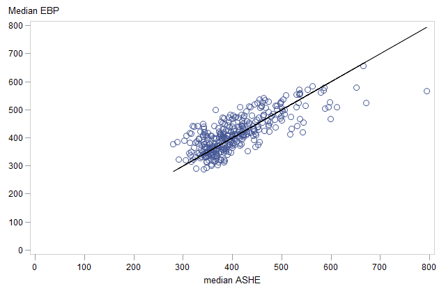
A similar analysis was also conducted for the mean and the other percentile estimates of income. Table 14 shows the correlations between the EBP local authority estimates and the corresponding ASHE estimates. For some local authorities the ASHE estimate was not of publishable quality due to a large coefficient of variation (CV) and these local authorities were removed from the comparison. For most estimates, this was a small number, however, for the 90th percentile only 64 (18%) of the local authorities gave acceptable CVs in the ASHE analysis. As a consequence, the 90th percentile is not included in Table 14.
The EBP local authority estimates of the mean and 75th percentiles both correlate highly with the corresponding ASHE estimates. The EBP local authority estimates of the 25th percentile have a moderately high correlation of 0.63, whereas the EBP local authority estimates of the 10th percentile have a somewhat weaker correlation of 0.45. These findings are discussed more in Section 7.
Table 14: Correlations between the 2011 EBP estimates and the corresponding 2011 ASHE estimates, local authority level
| Estimate | Sample size | Correlation between 2011 EBP estimates and 2011 ASHE estimates |
|---|---|---|
| 10th percentile | 318 | 0.45 |
| 25th percentile | 340 | 0.63 |
| Mean | 339 | 0.82 |
| Median | 340 | 0.77 |
| 75th percentile | 333 | 0.81 |
| Source: Office for National Statistics | ||
Download this table Table 14: Correlations between the 2011 EBP estimates and the corresponding 2011 ASHE estimates, local authority level
.xls (26.6 kB)6.3 Assessment against ONS 2011 to 2012 National Statistics (MSOA-level)
The Empirical Best Predictor (EBP) estimates are also assessed through comparison with the published ONS model-based mean household income estimates for 2011 to 2012. We currently produce model-based estimates of mean household income on a triennial basis and these are published as National Statistics.
Figure 13 shows the EBP mean household income estimates for 2011 plotted against the published ONS mean household income estimates for 2011 to 2012. Both estimates relate to all 7,201 Middle Layer Super Output Areas (MSOAs) across England and Wales and both are benchmarked to regional level estimates from the Family Resources Survey (FRS) (EBP estimates benchmarked to regional totals as opposed to the mean).
The estimates are highly correlated with no evidence of nonlinearity, as we would expect given that they are both benchmarked to regional level estimates from the FRS. The correlation coefficient between the two sets of estimates is 0.97. There is an approximate even distribution of points either side of the y equals x line meaning that neither the EBP nor the current estimates have a tendency for producing higher or lower estimates.
The same plot was also looked at for each English region and Wales. Similar conclusions were found in all plots with points approximately evenly distributed either side of the line y equals x.
The scaling factors used for benchmarking the published ONS estimates for 2011 to 2012 ranged from 0.92 (Wales) to 1.19 (London). It is important to note that for the published estimates the scaling factor has only been applied to the mean whereas the EBP approach also rescales percentiles of the income distribution.
Note that the published estimates are based on the log transformation and do not include household-level covariates in the modelling process, whereas the EBP method is based on a Box-Cox transformation and includes both household-level and MSOA-level covariates in the modelling process. Therefore, given the difference in methodologies, some differences are expected.
Figure 13: Estimated mean household weekly income (equivalised, after housing costs) at MSOA-level, 2011 EBP estimates versus 2011 to 2012 estimates derived using the current ONS method
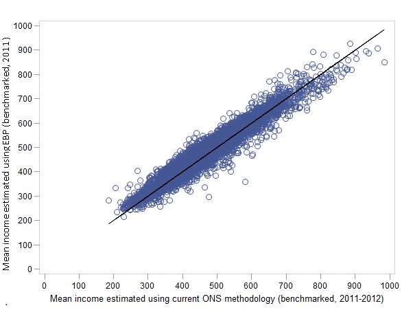
Source: Office for National Statistics
Download this image Figure 13: Estimated mean household weekly income (equivalised, after housing costs) at MSOA-level, 2011 EBP estimates versus 2011 to 2012 estimates derived using the current ONS method
.png (51.2 kB)
Figure 14 compares the coefficients of variation (CVs) for the EBP and published model-based estimates of mean household income. The median of the EBP CVs across all MSOAs is 0.050 as opposed to 0.067 for the published estimates. However, the CVs of the EBP estimates vary more with different MSOAs, which may in part be due to the nature of the bootstrapping method used to estimate uncertainty.
Figure 14: Comparison of coefficients of variation: 2011 EBP mean estimates and 2011 to 2012 ONS published mean estimates, MSOA-level
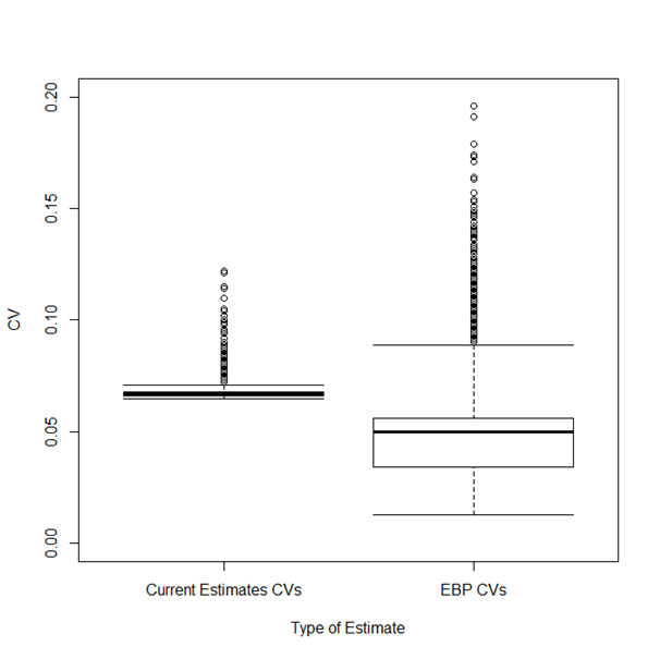
Source: Office for National Statistics
Download this image Figure 14: Comparison of coefficients of variation: 2011 EBP mean estimates and 2011 to 2012 ONS published mean estimates, MSOA-level
.png (23.9 kB)
7. Concluding remarks and future work
7.1 Discussion
Summary measures of household income at low-level geographies in England and Wales are required by users to better inform planning and decision-making. This work describes the use of the Empirical Best Predictor (EBP) method (Molina and Rao, 2010) to obtain model-based small area estimates of means, medians and percentiles for household income at Middle Layer Super Output Area (MSOA) level in England and Wales using the 2011 Census and the 2011 to 2012 Family Resources Survey (FRS) data.
This work shows four notable improvements over the initial application of the EBP approach at Office for National Statistics (ONS), as detailed in Small area estimates of income: means, medians and percentiles. Firstly, analyses are provided for more recent data since 2011 to 2012 FRS data and 2011 Census data are used as opposed to 2001 to 2002 FRS data and 2001 Census data.
Secondly, transformations of the income dependent variable were investigated to improve the model fitting for the multilevel model fitted to the FRS data. The chosen transformation was income raised to the power 0.2, which is based on a Box-Cox transformation. This transformation gave improvements in meeting model assumptions over the log transformation that was considered in Small area estimates of income: means, medians and percentiles.
Thirdly, Wales and all nine regions of England are considered in the analysis, as opposed to just the South East and North West regions of England.
Finally, the EBP estimates are benchmarked to regional direct estimates of total household incomes from the FRS, whereas the EBP estimates in Small area estimates of income: means, medians and percentiles are not benchmarked. This is the current best solution, as discussed in Section 3, since there is no established method for benchmarking percentiles directly.
Estimates of variability were presented in the form of coefficients of variation to help assess the quality of the estimates. For the MSOA-level estimates of mean household income, no coefficients of variation (CV) were greater than 0.20 and the median of these CVs was approximately 0.05 across all MSOAs, indicating that these estimates are of good quality. In official statistics, estimates with CVs greater than 0.20 are typically taken to be less reliable. Similar conclusions were found for the MSOA-level estimates of median household income.
For the upper extremes of the distribution, no CVs were greater than 0.20 and the median of the CVs was approximately 0.05 across all MSOAs for both the 75th and 90th percentiles. For the low extremes of the distribution (10th and 25th percentile), a small number of MSOAs had CVs over 0.20. However, the median CV across all MSOAs was approximately 0.06 for both the 10th and 25th percentiles.
Although the Annual Survey of Hours and Earnings (ASHE) estimates of employee income at local authority level are not directly comparable with the EBP estimates, the external validation conducted in Section 6.2 gave some confidence in the validity of the EBP estimates. However, the low correlation between the EBP 10th percentile estimates and the corresponding ASHE estimates, combined with the presence of some higher CVs for the EBP 10th percentile estimates, indicate that estimates in the very extreme of the distribution should be treated with more caution.
A further point to add is that the parametric bootstrapping method used for estimating the variability of the estimates assumes that the fitted FRS model captures the whole distribution of income. Although the Box-Cox transformation offers a notable improvement over the log transformation in terms of satisfying the normality assumption, the transformation is not perfect since the Q-Q plot given in Figure 2 shows that the extremes of the distribution are not fully captured. As a consequence, the CVs reported for the extremes of the distribution may be underestimated. Given all these points, the EBP 10th and 90th percentile estimates in particular should be treated with more caution than the other estimates produced in this report.
The ability to produce MSOA-level estimates of means and percentiles using the EBP approach was only possible due to being granted access to use the secure data environment at ONS where the household-level Census data are stored. The secure environment at ONS is extremely powerful, which was vital for the computational demands of the EBP approach. Obtaining the point estimates was relatively quick in the secure environment with computational time taking under 1 hour. However, the bootstrapping approach for obtaining estimates of variability was extremely computationally demanding and took over 120 hours.
This report has demonstrated that the MSOA-level estimates of means and percentiles obtained using the EBP approach are generally very accurate with low CVs. In addition, after benchmarking to regional totals from the FRS, estimates of mean household income at regional level for the EBP approach were found to match well with the corresponding direct estimates from the survey. A notable advantage of the EBP approach is that almost any statistic of interest can be estimated under one methodology.
7.2 Future work
The main area for future work is to assess the long-term potential of the Empirical Best Predictor (EBP) approach at Office for National Statistics (ONS). Model-based estimates of mean household income are currently produced as National Statistics using a different approach (see Section 3 for more information). The EBP approach offers percentile estimates for each MSOA as opposed to just the mean and therefore has potential to better meet user needs. Figure 13 shows that the EBP mean estimates were highly correlated with the official mean estimates with neither having a tendency for producing higher or lower estimates.
A limitation of the EBP approach is that household-level covariates are required in both census data and survey data, and so income estimates can only be derived in census years. Future work could consider how we can produce estimates between census years. This might include, for example, whether it is possible to update the census covariates or whether we could make more use of administrative data. However, even if no solution is found for the non-census years, the EBP estimates could still be beneficial as an additional output to accompany the 2021 Census.
Another potential area for further work is to investigate the benchmarking of the EBP estimates in more detail. Since there is no established method for directly benchmarking the percentile estimates, this report uses the best available solution whereby the estimates are benchmarked to direct survey estimates of regional totals. As well as assessing the effect of the current benchmarking method that has been implemented in more detail, it may be possible to implement a more sophisticated method in the future.
This report has only produced coefficients of variation (CVs) for the unbenchmarked estimates. Whilst these are believed to be similar to the benchmarked CVs and therefore a good representation of the variability of the benchmarked estimates produced in this report, it may be of interest to assess this assumption fully. To do this, a more sophisticated bootstrapping procedure is needed that ensures that each simulated bootstrap population has regional totals that match the FRS regional total direct estimates used for benchmarking the point estimates.
Nôl i'r tabl cynnwys8. Acknowledgements
Office for National Statistics is grateful to Nikos Tzavidis and colleagues at Southampton University for continuous advice and support throughout the production of this report.
Nôl i'r tabl cynnwys