1. Introduction
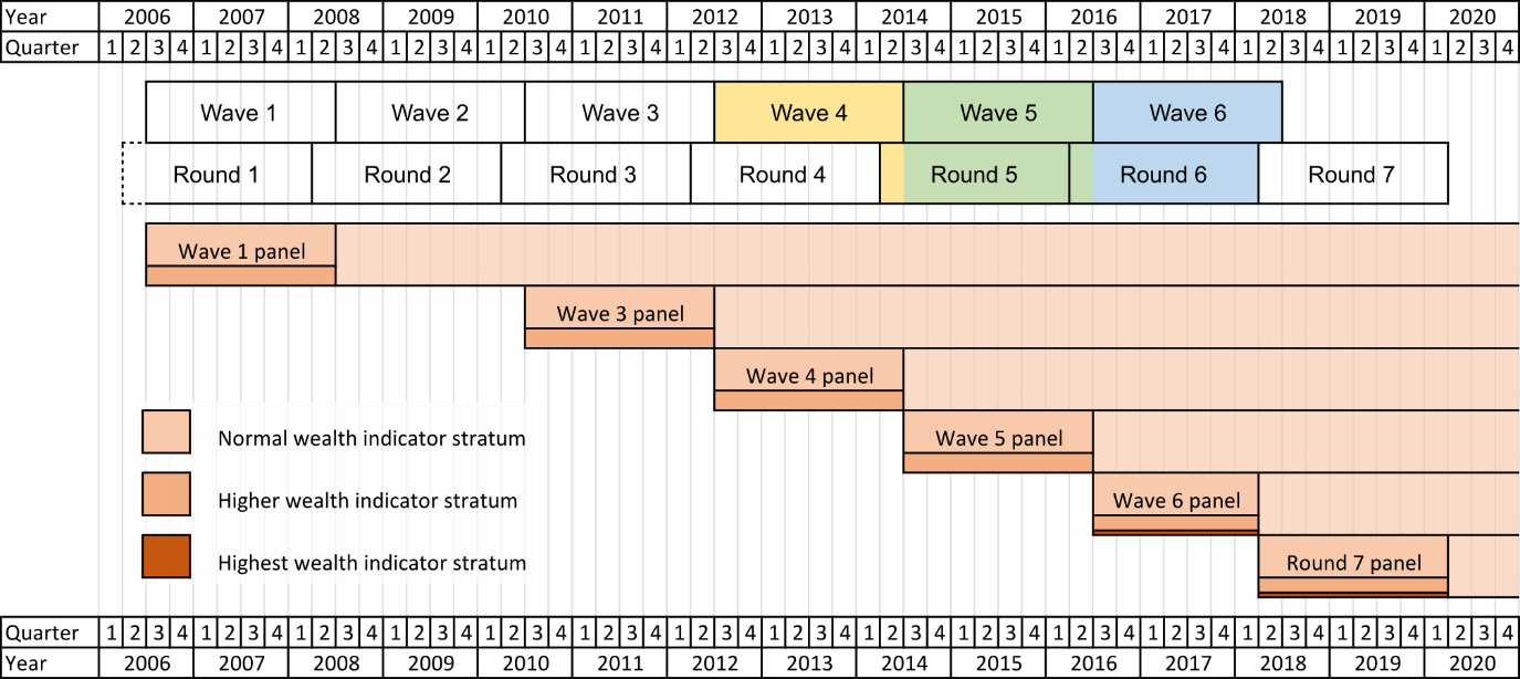
The Wealth and Assets Survey (WAS) is a biennial longitudinal household survey conducted by the Office for National Statistics (ONS). Covering Great Britain, the purpose of WAS is to "measure the well-being of households and individuals in terms of their assets, savings and debt and planning for retirement". Launched in 2006, the first five "waves" of the survey used 24-month reporting periods starting at the month of July of even years (the reporting period denotes the time window over which published survey estimates are computed). After the fifth wave of the survey, however, we decided to shift the reporting period by three months to begin in April, rather than July, so that it aligns with a financial-year periodicity. The first affected publication was the full two years of data starting in April 2016, called "round" six. Changing from waves to rounds required new methods for combining data from different periods and an adaptation of the established WAS weighting system. In particular, it had to accommodate the fact that the dataset for the financial-year-based round six (R6) comprised the final quarter of the mid-year-based wave five (W5) dataset and the first seven quarters from W6 (see Figure 1).
This article presents the new weighting system for WAS rounds. Conventionally, in a longitudinal survey, weights for a new reporting period are computed iteratively using the weights from the previous period as input. However, it would have been impractical to re-compute weights for rounds in this way starting from R1 and using only the raw weighting input data (rounds before R6 are formally defined by going back from R6 in two-year steps; round RT always comprises the last quarter of wave W(T-1) and the first seven quarters of WT; see Figure 1). Therefore, we developed a method to obtain R5 cross-sectional weights directly from existing W4 and W5 weights. Weights for R6 were then computed from the R5 weights using an adapted version of the established scheme for WAS waves. Modifications particularly affected the latest boost panel as well as the calibration procedure.
The article is organised as follows. After a brief summary of the WAS sample design and panel structure in Section 2, the method for constructing cross-sectional weights for WAS rounds directly from wave weights is presented in Section 3. The following sections describe the new round-based weighting system. As a first step, the longitudinal R5 to R6 person-level weights are derived (Section 4) followed by the computation of the cross-sectional R6 person- and household-level weights (Section 5). Section 6 discusses two further types of weights calculated for WAS: non-proxy and survivor weights. To assess the approach and to illustrate quality testing, Section 7 compares WAS estimates using R6 weights calculated under the new scheme to those using weights directly derived from waves five and six. A brief outlook on possible future developments and improvements of the weighting system is given in Section 8.
A detailed description of the weighting system for WAS waves was given in an earlier ONS Survey Methodology Bulletin paper by Davies (PDF, 1.55MB). This article should be considered as an update on this previous publication, rather than as a complete and self-contained presentation of the new system. As such, this article focuses in most places on a concise discussion of the main aspects while referring to Davies' paper for details of the mathematical description. Further information on the WAS weighting system can be found in the WAS User Guides.
Nôl i'r tabl cynnwys2. Sample design
Figure 1 summarises the historical development of the Wealth and Assets Survey (WAS) and illustrates the switch from waves to rounds. After the launch in July 2006, new boost panels were added to the survey in every wave starting from wave three (W3) in order to compensate for attrition. To construct a new panel, WAS uses a two-stage stratified cluster design. Primary sampling units (PSUs) are formed by postcode sectors. Until round seven (R7), they were drawn by stratified systematic sampling with probability proportional to size. Stratification variables comprised geographic region, metropolitan borough status, the proportion of households with the household reference person in National Statistics Socio-Economic Classification (NS-SEC) groups one to three and proportion of households without car. Starting from R7, PSUs are drawn from the PSUs used in the previous year's Survey of Living Conditions (SLC), which employs a similar stratification scheme.
A list of the selected PSUs is then submitted to HM Revenue and Customs (HMRC) where addresses likely to be in the top decile of wealthy households are identified based on tax return data. Within PSUs, these wealthy households are oversampled by a factor of three (from W6 onwards, the top percentile is oversampled by a factor of five). Further details on the sample design and a derivation of sampling probabilities are provided in Davies' Office for National Statistics (ONS) Survey Methodology Bulletin paper (PDF, 1.55MB) and the WAS User Guides.
After W5 (July 2014 for June 2016), the start of the reporting period was shifted by three months from mid-year to the beginning of the financial year and reporting of round-based results thus commenced with R6 (April 2016 to March 2018). R6 overlaps with the final quarter of W5 and the first seven quarters of W6. Note that individual households retain their two-year periodicity; a household interviewed in the final quarter of W5 (Quarter 2 2016) is interviewed again two years later in the first quarter of R7 (Quarter 2 2018).
Figure 1: Timeline of WAS showing panel structure and the timing of waves and rounds
Source: Government Statistical Service – Changes to the Wealth and Assets Survey weighting system because of a shift in the reporting period
Notes:
- The yellow, green and blue shadings illustrate how round five (R5) and R6 are composed of parts of waves four (W4) to six. Wealth strata are used for sample selection; the highest wealth stratum was only introduced in W6 (see text for details).
Download this image Figure 1: Timeline of WAS showing panel structure and the timing of waves and rounds
.png (143.5 kB)Survey weighting
With regard to survey weighting, the shift from waves to rounds posed several challenges.
As explained in Section 1, it was necessary to develop a method for combining weights across two consecutive waves; this method is presented in Section 3.
In the weighting scheme for waves, the various wave panels were processed separately before combining them at the end of the procedure. We have to consider how this approach should be adapted for the new scheme, whether the old panels should be retained or processing should be based on panels formed according to rounds, and whether it would be possible to combine some of the panels, as sizes decrease over time because of attrition. These issues are particularly relevant with regard to attrition modelling, which is done by panel. For the moment, the old wave-based panels have been retained (except for the new R6 panel, see Figure 3). However, attrition modelling for these panels considers changes between rounds, apart from the R2 to R6 survivor weights. These decisions might be revisited in subsequent rounds.
Sample sizes and numbers of respondents can vary considerably between panels and quarters. In the new scheme, the last step of the cross-sectional weighting procedure therefore combines panels within quarters by effective sample size and then calibrates the resulting datasets separately by quarter. Quarters are then collated to form the final set of weights.
Nôl i'r tabl cynnwys3. Starting up the round-based weighting system
Weighting a longitudinal survey such as the Wealth and Assets Survey (WAS) is an iterative process in which the weights computed for a given reporting period are used as input for the subsequent cycle. However, for practical reasons, it was not feasible to compute weights systematically for WAS rounds in this way, that is by starting "from the beginning" at round one (R1) and using only the raw input information. Therefore, a method was devised with which cross-sectional weights for any WAS round could be directly derived from the existing weights of the corresponding WAS waves. This method is described later for the example of obtaining R5 weights from the final quarter of wave four (W4) and the first seven quarters of W5. The R5 weights are then used as input to a "round-based" system to derive R6 weights.
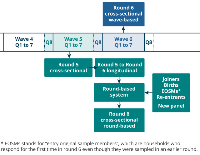
Besides computing R5 weights, the same method was also used to obtain "wave-based" R6 weights directly from W5 and W6 data (see Figure 2) for quality checking (see Section 7). R2 weights were required as a starting point for the production of round-based survivor weights (see Section 6: Survivor weights) and were also computed using the same method. If needed, it would also be possible to obtain R3 and R4 cross-sectional weights in this way, but this has not been done yet. Note that the R5 weights were used to compute wealth estimates in an Office for National Statistics (ONS) report on the switch from waves to rounds.
Figure 2: Derivation of round- and wave-based round six weights
Source: Government Statistical Service – Changes to the Wealth and Assets Survey weighting system because of a shift in the reporting period
Notes:
- The “wave-based” weights are directly obtained from wave five (W5) and W6 cross-sectional (XS) weights whereas the “round-based” weights are computed by applying the round-based system to the round five (R5) weights. Entry original sample members (EOSMs) are households who respond for the first time in R6 even though they were sampled in an earlier round.
Download this image Figure 2: Derivation of round- and wave-based round six weights
.png (32.8 kB)The approach to computing R5 weights from W4 and W5 proceeds as follows:
stage one: form quarterly datasets from the existing cross-sectional person weights for the final quarter of W4 and the first seven quarters of W5
stage two: calibrate each quarterly dataset to the midpoint of R5 (March 2015) using the age or sex and regional calibration groups already established for the weighting of WAS waves; calibration can be carried out to obtain person or household weights as detailed in Section 5: Person- and household-level cross-sectional weights
stage three: rescale each of the eight quarterly datasets by one-eighth and combine them to form the final R5 cross-sectional weights; in this way, the resulting weights are automatically calibrated to the R5 midpoint totals as well
The main reason for adopting this approach was to account for unequal sample sizes across quarters. We expect that the quarterly calibration will make the sample more representative over the eight quarters of the two-year reporting period. As a future refinement, we could calibrate each quarter to its own midpoint. This would make it easier to produce annual estimates (note that calibration to quarter midpoints was used in W1 but was dropped subsequently as WAS methods developed over time).
We chose to compute R6 weights starting from R5 weights using a round-based system, rather than simply only producing the "wave-based" R6 weights obtained from W5 and W6 cross-sectional weights. This is because the round-based system implements Verma, Betti and Ghellini's standard iterative weighting methodology for longitudinal data, as does the original system developed for WAS waves. Therefore, it appeared appropriate to develop this in R6 and use the comparison between wave- and round-based R6 weights for quality checking and have a working system to use from R7 onwards.
Nôl i'r tabl cynnwys4. Computing R5 to R6 weights based on R5 weights
Longitudinal round five (R5) to R6 weights are used to produce estimates for the R5 survey population at the time of R6. They differ from the R5 cross-sectional weights because of the loss of follow-up between rounds. They are both an output of R6 weighting as a final deliverable as well as a stepping-stone for computing R6 cross-sectional weights. In the round-based weighting system, they are obtained as follows:
stage one: separate the dataset for the R5 cross-sectional person weights into the original wave-based panels
stage two: for each panel, compute and apply attrition adjustments for drop-out from unknown eligibility and non-response between R5 and R6; the methodology for these adjustments is explained in an earlier Office for National Statistics (ONS) Survey Methodology Bulletin paper by Davies (PDF, 1.55MB) and Section 3 (see, for example, Equation (8)), and it is very similar to the procedure for Survivor weights described in Section 6, step 2
stage three: combine the panels based on their effective sample size (see Davies' paper, Section 3.2.1: Combining the panels), using the weights computed in step 2
stage four: form quarterly datasets and calibrate each to the midpoint of R5 (March 2015) using the standard calibration groups
stage five: rescale each of the eight quarterly sets by one-eighth and combine them to form the R5 to R6 longitudinal weights
Similar to the approach to computing cross-sectional weights for rounds from wave weights (see Section 3), calibration is performed on quarterly datasets, to account for varying sample size between quarters. As a slight alteration of the method, one could have also considered quarterly calibration within panels. However, this is often not feasible as longitudinal sample sizes become too small.
Nôl i'r tabl cynnwys5. R6 cross-sectional weights
This section first presents a description of the new round-based weighting system, followed by an explanation of how person- and household-level cross-sectional weights are computed.
Round-based weighting system
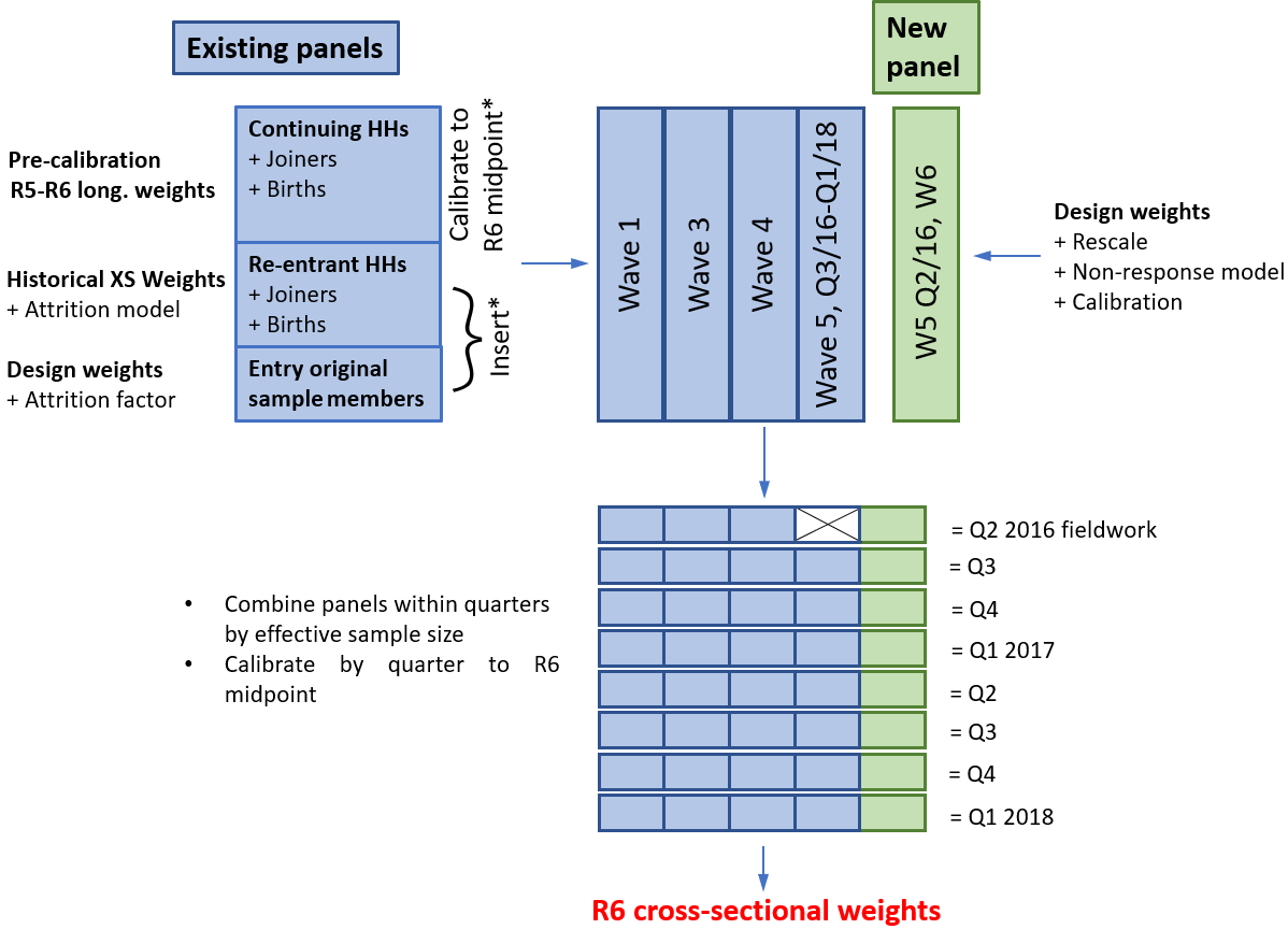
Figure 3 presents an overview of the round-based system for computing the round six (R6) cross-sectional weights. The overall structure of the approach is very similar to the one used to weight Wealth and Assets Survey (WAS) waves, as per Davies' Office for National Statistics (ONS) Survey Methodology Bulletin paper (PDF, 1.55MB). It should be noted that for the initial processing, cases are still grouped into the original wave-based panels (with the exception of the final quarter of wave five (W5), which is moved to the new panel). However, the attrition and non-response models for re-entrants and first-time respondents are constructed on a round basis. We expect that this system can easily be adapted to computing cross-sectional weights in future rounds.
Figure 3: Overview of the round-based system for computing the round six cross-sectional weights
Source: Government Statistical Service – Changes to the Wealth and Assets Survey weighting system because of a shift in the reporting period
Notes:
- The calibration and insertion steps for parts of the existing panels are explained in the text.
Download this image Figure 3: Overview of the round-based system for computing the round six cross-sectional weights
.png (77.8 kB)The main steps of the round-based approach are as follows.
Stage one: cases continuing from R5 are assigned their pre-calibration longitudinal R5 to R6 weights (output of stage two in the procedure of Section 4), and joiners and births to their households are included using the established methodology (see page 51 of Davies' paper). The resulting set of cases is then split into panels and each panel is calibrated to the R6 midpoint population totals (March 2017).
Stage two: because of the design of WAS and its follow-up rules, there are some households who respond for the first time in R6 even though they were sampled in an earlier round (for example, it may not have been possible to contact the household before). Such cases are known as entry original sample members (EOSMs). They are assigned a weight that is the product of their original design weight (that is, the reciprocal of their initial sampling probability) and an attrition factor. The reciprocal of this factor equals the estimated probability of an eligible case who was sampled in the same round as the EOSM to respond in R6. These probabilities are estimated separately for each geographic region and level of wealth index used for sampling (see Davies' paper, Equation (14)). Previously, the factor would have been computed using a wave-based attrition model.
Stage three: re-entrants (households who last responded prior to R5) are assigned a weight that is the product of their last cross-sectional weight and an attrition factor. This factor is computed from a round-based logistic regression model that describes the attrition rate within the re-entrant's panel, between the round that the re-entrant last responded in and the current round.
Stage four: EOSMs and re-entrants are added into their respective panels by appropriately shrinking the calibrated weights of the continuing households (see Davies' paper, Equation (15)).
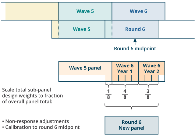
Stage five: the computation of the weights for the new panel (that is, cases sampled in R6) makes use of a procedure that accounts for differing sample sizes between subpanels (see Figure 4). In particular:
assign each case their original design weight
rescale the design weights for the last quarter of W5, the first four quarters of W6 and the fifth to seventh quarters of W6, respectively, to one-eighth, four-eighths and three-eighths of the R6 midpoint population total
apply a non-response adjustment computed from a logistic regression model for response propensity; the model considers all households sampled in R6 and estimates response probability using output area classification, region and the WAS wealth index as predictors
calibrate the panel to the R6 midpoint population totals
Figure 4: Processing of the new round 6 panel
Source: Government Statistical Service – Changes to the Wealth and Assets Survey weighting system because of a shift in the reporting period
Download this image Figure 4: Processing of the new round 6 panel
.png (24.7 kB)Stage six: quarterly datasets are formed by combining all panels by effective sample size within quarters.
Stage seven: the quarterly datasets are re-calibrated to the R6 midpoint population totals. Two different calibration schemes are used to obtain person- and household-level weights (see Section 5: Person- and household-level cross-sectional weights for details). Combining the quarters (and scaling weights by a factor of one-eighth) yields the final round-based R6 cross-sectional weights.
The wave-based panels were retained because a round basis would have led to three truncated panels: as shown in Figure 1, the R1 and R3 panels cover only seven quarters each (the first seven quarters of W1 and W3, respectively) whereas the R2 panel consists of a single quarter (the final quarter of W1). In contrast, with wave-based panels, only the W5 panel will be truncated to seven quarters.
As to attrition modelling, it could be argued that it might be more accurate to compute attrition for wave-based panels on a wave level. The switch to round-based modelling allows simplification of the code structure and avoids the need for multiple types of models in future rounds.
Person- and household-level cross-sectional weights
The WAS weighting scheme produces two different sets of cross-sectional weights. In the person-level set, each individual case receives their own weight. Person-level weights serve as starting points for deriving longitudinal and non-proxy weights, but they are not used for computing any estimates from WAS variables. These are defined at household level and hence household weights are used. Exceptions are estimates from questions on opinion and asset ownership, which are computed with non-proxy weights (see Section 6: Survivor weights).
The only difference in the derivation of person- and household-level weights is in how the final calibration stage of the weighting system is carried out; in particular, in both cases the quarterly datasets obtained in stage six of the procedure in Section 5: Round-based weighting system are used as input to the calibration. The calibrated person-level weights WPers,i have to fulfil constraints of the type
in each calibration group. Here, the summation extends over all individual household members, and is an indicator taking the values one or zero depending on whether the person is part of the calibration group or not.
For the household-level weights WHH,h, the same calibration groups are used but the constraints are now of the form
Here, the summation is over all households in the round, and denotes the number of household members in the calibration group in question. The input (pre-calibration) weights are the means of the person-level pre-calibration weights within households.
Nôl i'r tabl cynnwys6. Further sets of weights
In addition to cross-sectional and R(T-1) to RT longitudinal weights, two further sets of weights are usually produced in a Wealth and Assets Survey (WAS) reporting period: non-proxy and survivor weights. The procedures for computing these weights are briefly summarised in this section.
Non-proxy weights
WAS aims to conduct face-to-face interviews with all individuals in a household aged 16 years and older. However, for some adults, information is only obtained via proxy responses given by another household member. Certain WAS analyses disregard such proxy data and only consider responses from non-proxy cases. One particular example is provided by early publications of results from ongoing reporting periods, for example, using the first 6, 12 or 18 months of data. At this stage, imputation of WAS wealth variables has not yet taken place and interest focuses on opinion questions and information regarding asset ownership (see Section 2 of Early indicator estimates from the WAS: attitudes towards saving for retirement, automatic enrolment into workplace pensions and financial situation, July 2016 to December 2017).
Non-proxy analyses make use of a specifically derived set of weights. These are obtained by first computing standard person-level cross-sectional weights for the full set of available cases (for early indicator analyses, this would include all households interviewed before the cut-off date). The subset including all non-proxy cases and children below 16 years of age is then formed. (Note that children are indirectly covered in the interview process through proxy information given by parents. They need to be included in the survey as they can possess their own assets.) The cross-sectional person weights of this subset are re-calibrated in the usual way using the established calibration groups and the relevant population totals. Calibration takes place in a single step including all cases rather than separating the dataset into panels or quarters.
Survivor weights
Besides longitudinal weights for consecutive waves, for example, wave four (W4) to W5, WAS also provided so-called W1 to WT "survivor weights" for the initial W1 sample in all subsequent waves T up to W5. With the change from waves to rounds, we decided to replace these weights by round two (R2) to RT survivor weights. R2 was chosen as the basis for the weights rather than R1 as the latter covers only seven quarters of sampling (see Section 5 of Moving the WAS onto a financial years' basis).
As explained later in this section, the computation of survivor weights only needs to consider cases who responded in every period or have become ineligible at some point. Complications from joiners, re-entrants or additional panels therefore do not arise. Hence, it was feasible to compute R2 to RT weights for all T>2 in a round-based way starting from the R2 person-level cross-sectional weights. The calculation is based on an iterative algorithm where R2 to RT weights are used as input to derive the R2 to R(T+1) weights.
The scheme proceeds as follows.
Stage one (R2 weights): R2 person-level cross-sectional weights are computed for all R2 responders following the procedure outlined in Section 3.
Stage two (R2 to R3 weights): every R2 responder is classified according to their R3 response status as either R3 responder (R), ineligible case (IE), non-responder (NR) or case with unknown eligibility (UE). R3 ineligible cases are those who do not fulfil the R3 sample inclusion criteria, for example, because of death or emigration. Non-responders are known to be still in the R3 population but were not productive in R3, most often because of refusal. For some cases, R3 eligibility cannot be established, for example, if the current location of the household is unknown.
If there were no NR and UE cases, the original R2 population would be faithfully represented by the R3 R and IE cases, and no reweighting would be necessary. To deal with attrition, a two-step process is applied. First, UE attrition is handled by deriving an adjustment factor from suitably defined logistic regression models with eligibility as outcome (more precisely, unknown versus known eligibility) and fitted using all R2 responders. NR attrition is similarly addressed with the help of logistic regressions with response versus non-response as outcome and fitted using the R3 responders and non-responders. After applying the attrition adjustments (reciprocals of the response probabilities predicted by the logistic regressions) to their R2 cross-sectional weights, the R and IE cases are calibrated to the R2 population totals. Note that IEs only receive the UE attrition adjustment, while R3 Rs obtain both UE and NR adjustments (compare with Davies' Survey Methodology Bulletin paper (PDF, 1.55MB), Equation (6)). Consistent with the methodology for other types of weights for WAS rounds, calibration is performed on a quarterly basis.
Stage three (R2 to R4 weights): as a first step, cases who responded in both R2 and R3 are classified according to their R4 response status. Using the approach of stage two, the R2 to R3 weights of the R4 Rs and IEs are then adjusted for R4 attrition. Their new weights are combined with the unadjusted R2 to R3 weights of the R3 IEs and the complete set is calibrated to the R2 population totals.
Stage four (R2 to R5 and R2 to R6 weights): the R2 to R4 weights of R5 Rs and IEs are adjusted for attrition between R4 and R5 and then combined with the R2 to R4 weights of the R2 and R3 IEs before calibration to R2 population totals. R2 to R6 weights are computed accordingly.
It should be noted that the logistic regression models describing attrition are computed on a wave rather than a round basis. For example, R2 to R3 attrition factors for Quarter 1 of R2 (first quarter of R2, which coincides with the last quarter of W1, Quarter 8 W1) cases are computed using the regression models developed for W1to W2 weights (model fitting includes cases from W1, Quarters 1 to 7). In contrast, attrition factors for Quarters 2 to 8 R2 are based on the W2 to W3 models. Alternatively, one could have used a single R2 to R3 model for both groups. However, it seems that attrition for Quarter 1 R2 cases who had only their second chance of responding in R3 is better modelled by the W1 to W2 model in which every participant is in the same situation. In the R2 to R3 model, Quarter 1 R2 responders would be mixed in with a large majority of cases who already have their third chance of responding in R3. As attrition for W2 to W3 is probably lower than for W1 to W2, the resulting adjustments for Quarter 1 R2 would likely be too small.
While it was feasible to implement this more complex way of attrition modelling for survivor weights, it would have been too cumbersome to maintain a similar approach for cross-sectional and round-to-round longitudinal weighting involving multiple panels. Therefore, they make use of a simpler round-based system.
Nôl i'r tabl cynnwys7. Comparing wave- and round-based R6 weights and WAS estimates
In this section, we present some results of the round- and wave-based approaches (see Section 3) to computing cross-sectional round six (R6) weights. Besides directly contrasting the two sets of weights, we also compare estimates for various Wealth and Assets Survey (WAS) variables.
The round-based approach starts by constructing R5 cross-sectional weights from the existing weights for the final quarter of wave four (W4) and the first seven quarters of W5, using the method described in Section 3. One then applies the round-based system presented in Section 4 and Section 5 to compute longitudinal R5 to R6 and cross-sectional R6 weights (see Figure 1). In the wave-based approach, the cross-sectional R6 weights are directly computed from W5 and W6 weights, again using the method of Section 3.
Round- and wave-based R6 cross-sectional weights
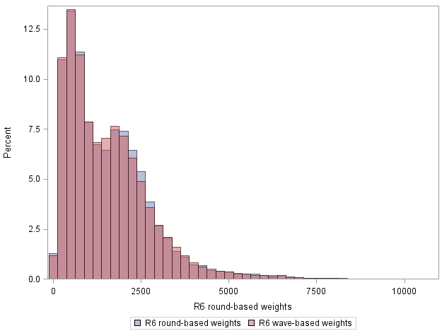
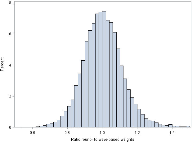
Basic comparisons between round- and wave-based cross-sectional person weights are presented in Table 1, Figure 5 and Figure 6.
| Type of weight | N | Sum | Minimum | Maximum | First percentile | 99th percentile | Coefficient of variation |
|---|---|---|---|---|---|---|---|
| Round-based | 40,540 | 62,933,121 | 18 | 9262.5 | 115.7 | 5731 | 0.763 |
| Wave-based | 40,540 | 62,933,121 | 16 | 10733 | 116.7 | 5756 | 0.772 |
Download this table Table 1: Summary statistics for round- and wave-based round six cross-sectional person weights
.xls .csv
Figure 5: Distributions of round-based (blue) and wave-based (red) R6 cross-sectional person weights shown as overlapping histograms
Source: Government Statistical Service – Changes to the Wealth and Assets Survey weighting system because of a shift in the reporting period
Download this image Figure 5: Distributions of round-based (blue) and wave-based (red) R6 cross-sectional person weights shown as overlapping histograms
.png (11.5 kB)
Figure 6: Histogram of the ratio of round- to wave-based weights
Source: Government Statistical Service – Changes to the Wealth and Assets Survey weighting system because of a shift in the reporting period
Download this image Figure 6: Histogram of the ratio of round- to wave-based weights
.png (11.6 kB)As shown in Table 1 and Figure 5, the distributions of round- and wave-based weights are very similar overall, even at the high-end tail. The bimodal structure seen in Figure 5 is a result of cases in the higher-wealth strata receiving smaller weights because of oversampling. The round-based weights have marginally higher precision (coefficient of variation 0.763 versus 0.772). Figure 6 shows the ratio of round- to wave-based weights. The ratio has a mean of 1.01 and a standard deviation of 0.19; for 90% of cases, it is between 0.82 and 1.21. The Pearson correlation between the two sets of weights is 0.979.
Note that because the target population of WAS are private households in Great Britain, the sum of the weights in Table 1 (62,933,121) represents an estimate of the corresponding population total for March 2017, the mid-point of R6. This means that the total represents the whole Great Britain population excluding individuals living in communal establishments such as halls of residence and care homes. The figure was derived by linear interpolation from available mid-year estimates for 2016 and 2017. The sum of weights for the round- and wave-based approach agree since both are calibrated to the same population totals.
Comparison of WAS estimates
The following tables show statistics for some WAS variables computed using both wave- and round-based cross-sectional household weights. To put the difference between the estimates into perspective, some results from previous waves and rounds are also included (W6 results are based on 21 months of data). Moreover, for the wealth estimates (Table 3), the difference between the round- and wave-based estimates is related to the sampling precision as measured by the standard error. Note that the estimates shown in the following tables were directly derived from raw data and therefore may differ from published values.
| Tenure Type | W4 | R5 | W5 | R6 RB | R6 WB | W6 |
|---|---|---|---|---|---|---|
| Owned outright | 32.53 | 32.53 | 32.66 | 33.48 | 33.55 | 33.49 |
| Buying with help of mortgage / loan | 33.47 | 33.11 | 32.95 | 32.38 | 32.26 | 31.99 |
| Part rent part mortgage (shared ownership) | 0.40 | 0.49 | 0.47 | 0.42 | 0.41 | 0.43 |
| Rented | 32.50 | 32.80 | 32.77 | 32.54 | 32.59 | 32.91 |
| Live here rent-free | 1.12 | 1.06 | 1.14 | 1.19 | 1.18 | 1.18 |
Download this table Table 2: Estimated distributions (percentage splits) of housing tenure types for WAS W4, R5, W5 and R6 using round- and wave-based weights, 21-months W6
.xls .csv
| Wealth component (£ trillion) | W5 | R6 RB | R6 WB | Relative difference R6 RB to WB [%] | (RB-WB) / SE [%] |
|---|---|---|---|---|---|
| Property Wealth (net) | 4.50 | 5.09 | 5.11 | -0.38 | -18.95 |
| Financial Wealth (net) | 1.84 | 2.12 | 2.15 | -1.09 | -5.25 |
| Physical Wealth | 1.25 | 1.32 | 1.32 | -0.14 | -13.15 |
| Private Pension Wealth | 5.36 | 6.10 | 6.10 | -0.01 | -0.95 |
| Total Wealth (incl. Pension) | 12.95 | 14.63 | 14.67 | -0.31 | -9.02 |
| Total Wealth (excl. Pension) | 7.59 | 8.53 | 8.57 | -0.52 | -9.14 |
Download this table Table 3: Estimates of main wealth components (in trillion GBP) for WAS W5 and R6 using round- and wave-based weights
.xls .csvFor tenure (Table 2), round- and wave-based results show only very small differences in the proportions of the various groups (0.1 percentage points or less) which are much less than typical changes between waves. Very similar behaviour was found for the other two categorical variables that were considered but not shown here: household composition and socio-economic classification (National Statistics Socio-Economic Classification (NS-SEC)).
For the main WAS wealth components, the relative differences between the R6 estimates obtained using round- and wave-based weights were about 1% or less (Table 3). Because of the small size of the differences and the complexity of the weighting scheme, it would be difficult to precisely identify the source of the discrepancies. Relative to the standard error of the estimates (computed using the generalised linearised jack-knife method), the differences between round- and wave-based estimates were between 1% and 19% in magnitude, which means that the impact on statistical inference would be negligible. Note that in Table 3, the round-based estimates are always smaller than the wave-based ones. However, this pattern does not hold for other variables that were investigated.
Nôl i'r tabl cynnwys8. Conclusions
The shift of the Wealth and Assets Survey (WAS) reporting period from waves to rounds necessitated some changes to the established survey weighting scheme. This article described the new system and discussed some of the considerations that informed its development. For example, calibration now takes place by quarters (except for non-proxy weights) to ensure that the system is more robust with respect to changes in numbers of respondents over time. Quality testing of the new scheme has shown that it works effectively and reliably so that we are confident that it is ready to be used for the next rounds of the survey. Nevertheless, there is still potential for further development and improvement of the weighting scheme. Some of the areas that we plan to consider and work on in the future include:
the way of handling the new panel was strongly affected by the switch from waves to rounds and thus is specific to round six (R6); the method will have to be modified again for future rounds
calibration to population totals for quarter midpoints rather than round midpoints; this should make it easier to produce annual estimates
in the calibration procedure for household weights, household totals for geographic regions could be introduced as an additional constraint; it needs to be investigated how this change would affect WAS estimates
the number of WAS panels increases with every new round, but at the same time individual panels decrease in size because of attrition; to simplify and stabilise the weighting procedure, we need to examine whether some individual panels can be combined into larger groups
for the future, we propose to integrate WAS into the Household Finance Survey (HFS), which will require further investigation (see Section 2 of Moving the WAS onto a financial years' basis); if the integration goes ahead, it will be necessary to harmonise the weighting schemes for the surveys
The authors, Oliver Zobay, Eleanor Law and Salah Merad, thank Dr Gareth James for very helpful comments and suggestions on an earlier version of the manuscript.
Nôl i'r tabl cynnwysManylion cyswllt ar gyfer y Methodoleg
philip.lowthian@ons.gov.uk /oliver.zobay@ons.gov.uk
Ffôn: +44 (0)207 592 8640 / +44 (0) 1633 456212
