Cynnwys
- Authors
- Main points
- Introduction
- Management practices and productivity of family-owned businesses
- Transforming turnover: using VAT turnover data in the national accounts
- Improvements to early estimates of GDP through the 2008 to 2009 downturn
- Understanding the UK economy
- Annex A – Publication dates and themes for future Economic reviews
- Annex B - Demand and supply indicators
2. Main points
A new survey on management practices shows family-owned businesses are associated with lower than average productivity at the firm level.
The development of VAT data within national accounts will significantly improve the coverage of smaller businesses in the measurement of gross domestic product (GDP).
Analysis of GDP estimates during the 2008 to 2009 economic downturn have led to improvements in the way we are using additional data, including VAT data to validate information available from monthly surveys.
GDP growth is estimated at 0.7% for Quarter 4 (Oct to Dec) 2016, Germany was the fastest growing G7 economy for 2016 as a whole.
The current account deficit improved in Quarter 4 2016, mainly due to an improved primary balance and an improved trade in goods position.
Most short-term output indicators slowed in January 2017 but show positive growth over the most recent 3 months.
Rising consumer prices, including owner occupiers’ housing costs (CPIH), are reflecting higher import prices, oil and fuel price increases and other factors such as a return to slight food price inflation over the last year.
3. Introduction
This edition of the Economic review is the first following the introduction of Economic Statistics Theme days in January this year. Each Economic review in this new format will have an overarching analytical theme and follow a quarterly publication timetable. The next edition is due for publication on 10 July 2017. Annex A provides information on the next 3 editions of the Economic review and their provisional theme.
Each review will also highlight progress being made to develop improved methods and statistics, which reflect the modern economy in line with the recommendations in the Independent review of UK economic statistics final report (Bean Review).
The theme of this Economic review is analysis of micro-data to investigate issues relating to the “productivity puzzle”. In particular, this review focuses on how a new survey of management practices in Great Britain is shedding light on differences in productivity, measured by output per worker, at the firm level.
The rest of the review discusses:
developments in the use of VAT data to estimate turnover of businesses for inclusion in the national accounts
gross domestic product turning points, using evidence from 2008 to 2009, and highlights the potential for VAT data to improve estimates of GDP
the economic data released since early December 2016 (the date of the last Economic review); this section will cover the Quarterly National Accounts and associated releases for Quarter 4 2016, prices and employment data, and indicators of production, construction, retail sales, services and trade covering the first 2 months of 2017. Data on the performance of the UK economy can also be found in the dashboard for understanding the UK economy.
4. Management practices and productivity of family-owned businesses
Introduction
Over recent years the UK has experienced low productivity growth and low levels of labour productivity relative to countries such as Germany and the US. At the same time, a growing body of research into productivity performance has provided evidence across a wide range of countries that better management can explain why some businesses perform better (for example, Bloom et al. 2014).
In response, the Office for National Statistics (ONS) set up the pilot Management Practices Survey (MPS) in 2016 to investigate the relationship between management practices and labour productivity in the UK. In our analysis, we find that most businesses in our manufacturing population are small, domestic or family-owned. We find these types of business having relatively low management practice scores, indicating lower use of structured management practices. We also establish an association between higher management practice scores and higher levels of labour productivity. For family-owned businesses, however, we find that they perform significantly poorer than non-family owned businesses in terms of labour productivity, irrespective of their management score.
Background of survey
The MPS pilot was a voluntary survey of 1,026 manufacturing businesses within Great Britain, with employment of 10 or more. The survey achieved a 68% response rate (702 responses). To measure the prevalence of structured management practices within a business, the survey asked eight main questions on a range of practices, including key performance indicators, targets, hiring decisions, promotions and managing staff under-performance. We translated these responses into a single management score by scoring responses to each question between 0 and 1 where 0 indicated the least structured management practices and 1 indicated the most structured management practices. These question scores were then averaged to give an overall management score for each business. Further details of these questions and how the answers were scored are available in Annex 3 of Awano et al. (2017).
In addition to the management questions, the survey also collected information on multinational status, family ownership and family management, to allow us to examine whether these business structures tend to use different management practices and whether these are associated with their productivity.
The manufacturing business environment
Within our population of interest – manufacturing businesses with employment of 10 or more – we find that around two-thirds (64%) of these businesses have some kind of family-ownership (which includes being owned by the founder of the business) and over half (55%) of the business population have a Managing Director who is either an owner or related to the owner; we refer to these businesses as being family-owned and family-managed (Figure 1c). Figures 1a and 1b show that just under three-quarters (74%) of businesses are small – with employment between 10 and 49, and more than 8 in every 10 businesses (84%) have no offices or operations outside of the UK – we term these domestic businesses. This business demographic plays an important role in understanding the scale and impact of the prevalence of structured management practices within the population and the association with labour productivity.
Figure 1a: Share of manufacturing businesses by characteristic, multinational status
Great Britain, 2015
Source: Office for National Statistics
Notes:
- Population of interest is manufacturing firms with employment of at least 10 in Great Britain.
Download this chart Figure 1a: Share of manufacturing businesses by characteristic, multinational status
Image .csv .xls
Figure 1b: Share of manufacturing businesses by characteristic, size
Great Britain, 2015
Source: Office for National Statistics
Notes:
- Population of interest is manufacturing firms with employment of at least 10 in Great Britain.
Download this chart Figure 1b: Share of manufacturing businesses by characteristic, size
Image .csv .xls
Figure 1c: Share of manufacturing businesses by characteristic, family ownership
Great Britain, 2015
Source: Office for National Statistics
Notes:
- Population of interest is manufacturing firms with employment of at least 10 in Great Britain.
Download this chart Figure 1c: Share of manufacturing businesses by characteristic, family ownership
Image .csv .xlsAverage management practice scores and productivity by business type
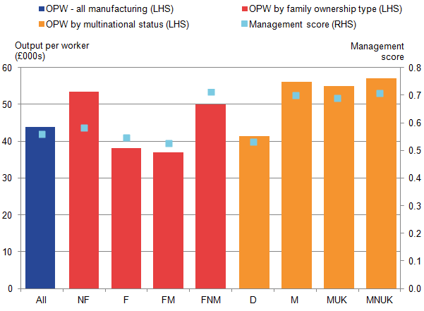
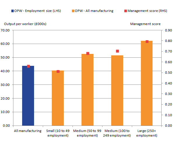
From the Management Practice Survey (MPS) results presented in Figure 2, we find average management scores higher among non-family owned businesses and multinationals1. Within family-owned businesses, those managed by non-family members score significantly higher than those with an owner or family member as the Managing Director. Conversely, groups that make up large shares of the manufacturing population, that is, domestic and family-owned and -managed businesses have relatively low scores, indicating lower prevalence of structured management practices in these businesses. We also find the use of structured management practices to be lowest among small businesses (employment of 10 or more) and increasing as business size increases (Figure 3).
Using linked financial data from the Annual Business Survey (ABS) for these businesses, we are able to examine the relationship between management practice scores and levels of labour productivity (Figure 2 – left hand side). We find a positive relationship between more structured management practices and higher levels of productivity. A notable point from this result is that family-owned businesses with family-led management had the lowest management practice scores and levels of productivity across all business types.
Figure 2: Labour productivity and management score by family ownership
Great Britain, 2015
Source: Office for National Statistics
Notes:
- OPW is output per worker.
- Labour productivity is measured as output per worker (GVA/employment) in 2015 current prices.
- Population of interest covers manufacturing business in Great Britain with employment of at least 10.
- Key:
All is All manufacturing (for businesses with at least 10 in employment)
NF is Not family-owned.
F is Family-owned.
FM is Family-owned and family-managed.
FNM is Family-owned and non-family-managed.
D is Domestic.
M is Multinational.
MUK is Multinational with head office based in the UK.
MNUK is Multinational with head office based outside the UK.
Download this image Figure 2: Labour productivity and management score by family ownership
.png (21.7 kB) .xls (21.5 kB)
In Figure 3, we examine the relationship between management practice scores and levels of labour productivity for businesses in different size groups. We also find here a positive relationship between management practice scores and levels of labour productivity. Since the majority of businesses in our population are either family-owned and managed, domestic or small (10 to 49 in employment), we begin to establish a pattern that suggests that there is some relationship between management scores and levels of labour productivity.
Figure 3: Labour productivity and management practice score by firm size
Great Britain, 2015
Source: Office for National Statistics
Notes:
- OPW is output per worker.
- Labour productivity is measured as output per worker (GVA/employment) in 2015 current prices.
- Population of interest covers manufacturing business in Great Britain with employment of at least 10.
Download this image Figure 3: Labour productivity and management practice score by firm size
.png (17.2 kB) .xls (26.6 kB)
Estimating relationships between management practice scores and business types
We use regression analysis to estimate the strengths of the relationships between management practices and the various business characteristics, and between labour productivity, business characteristics and management practice scores (Table 1).
In the first two columns of Table 1 we investigate how management score varies across businesses in different employment size groups and business types. The results can be interpreted as indicating that businesses that are 10% larger have management scores that are 0.11 higher. This is consistent with the trend we observe in Figure 3, showing management practice scores increasing as the employment sizes get larger.
We also established in the previous descriptive analysis (Figure 2), that within family-owned firms, those managed by non-family members had significantly higher management scores compared with those managed by members of the owning families. In our regression however, this pattern is not replicated. In column 2, we do not find any significant differences in management scores for family-owned firms, whether family-managed or not, once we have accounted for size, industry, multinational status and business’s age.
Estimating relationships between management practice scores and productivity
Similarly to the previous analysis, in columns 3 to 5, we use regressions to better understand the pattern we observe on the relationship between management practice scores and labour productivity. We start with a simple model and gradually add more variables to the model, in order to examine the effect of each additional variable(s) on the strength of the association from the initial position.
Our first model, in column (3) of Table 1, examines the unconditional relationship between management score and labour productivity. It shows that with the management score on a scale of 0 to 1, a 0.10 increase in score is associated with an 8.6% increase in labour productivity. To put this in context, the distribution of management scores shows that there is a 0.13 difference in score between the median and the 75th percentile, so this relationship translates to a difference in productivity of 11.1%2. Overall, this simple model estimates that management score accounts for 8% of the variation in productivity across businesses.
When we hold constant (control for) employment size and industry, the model in column (4) shows a reduced magnitude of the relationship between management score and productivity, so that a 0.10 increase in management score is associated with a 6.1% increase in labour productivity. Perhaps surprisingly, size plays a relatively small role, as the coefficient for size is not highly significant and only corresponds to an increase of 5% in labour productivity for a doubling in employment.
When we add variables for family business types, multinationals and business age (column 5), we find that a 0.10 increase in management score is associated with a 6.7% rise in productivity, translating to a difference in productivity of 8.7% between the median management score and the 75th percentile. Together, all factors included in the regression account for just over a fifth of the variation in productivity at the business level.
In this final model (column 5), it also emerges that family-owned businesses, both with and without family management, have much lower productivity, once we control for management score, size, industry, age and multinational status. While the coefficients for these two family-owned business types differ in magnitude, that difference is not statistically significant, so we conclude that productivity is around 20% lower for these family-owned businesses in general.
Given that family-owned businesses account for around three-quarters (64%) of businesses in our population of interest, this prompts further questions about why these businesses are performing relatively poorly. Chrisman et al (2017) for instance suggest that family-owned firms may be facing some adverse selection problems in the labour market, as more competent workers are attracted to non-family-owned firms, which offer better incentive compensation. While our results on the relationship between management practices and productivity cannot confirm that more structured practices have a direct impact on performance, they do suggest that this could be confirmed through further work. If so, family-owned businesses could have a mechanism through which they could improve, even if it is not possible to fully understand their current relatively poor performance.
Table 1: Regression analysis of management score and labour productivity at the business level
| Great Britain, 2015 | ||||||
| (1) | (2) | (3) | (4) | (5) | ||
| Management score | Management score | Log (Output per worker) | Log (Output per worker) | Log (Output per worker) | ||
| Management score | 0.855** | 0.608** | 0.669*** | |||
| (0.312) | (0.29) | (0.226) | ||||
| Log(employment) | 0.110*** | 0.108*** | 0.049* | 0.047 | ||
| (0.012) | (0.014) | (0.027) | (0.042) | |||
| Family-owned and family-managed business | -0.006 | -0.184*** | ||||
| (0.058) | (0.067) | |||||
| Family-owned and non-family-managed business | 0.047 | -0.265*** | ||||
| (0.033) | (0.095) | |||||
| Multinational | 0.004 | -0.09 | ||||
| (0.043) | (0.105) | |||||
| UK Multinational | 0.002 | -0.08 | ||||
| (0.028) | (0.115) | |||||
| Age (years) | (0.000) | 0.017 | ||||
| (0.012) | (0.068) | |||||
| Age squared | (0.000) | (0.000) | ||||
| (0.000) | (0.002) | |||||
| Industry group dummies | Yes | Yes | No | Yes | Yes | |
| R2 | 0.327 | 0.336 | 0.079 | 0.184 | 0.216 | |
| Adjusted R2 | 0.319 | 0.322 | 0.077 | 0.171 | 0.195 | |
| Equal family p-value | 0.115 | 0.507 | ||||
| Joint industry p-value | 0.000 | 0.000 | 0.000 | |||
| Observations | 694 | 694 | 591 | 591 | 591 | |
| Source: Office for National Statistics | ||||||
| Notes: | ||||||
| 1. Standard errors in parentheses are clustered by industry and employment size band, * p < 0.1, ** p < 0.05, *** p < 0.01 | ||||||
| 2. All regressions use Ordinary Least Squares. A constant is also included in all regressions. | ||||||
| 3. “Equal family p-value” is the probability that coefficients for “Family-owned and family-managed business” and “Family-owned and non-family-managed business” are equal, and “Joint industry p-value” is the probability that the coefficients for all the industry grouping dummies are zero. These probabilities are estimated using F-tests. | ||||||
| 4. Labour productivity is measured as output per worker (GVA/employment) in current prices (for year 2015). | ||||||
| 5. Population of interest covers manufacturing businesses in Great Britain with employment of at least 10. | ||||||
| 6. Industry dummies are as follows: Food, beverages, tobacco (divisions 10 to 12); Textiles, wearing apparel, leather (divisions 13 to 15); Wood, paper products, printing (divisions 16 to 18); Chemicals, Pharmaceuticals, rubber, plastics, non-metallic minerals (divisions 20 to 23); Basic metals, metal products (divisions 24 to 25); Computer etc. products, electrical equipment (divisions 26 to 27); Machinery, equipment, transport equipment (divisions 28 to 30); Coke, petroleum, other manufacturing (divisions 19 and 31 to 33). | ||||||
Download this table Table 1: Regression analysis of management score and labour productivity at the business level
.xls (33.3 kB)Conclusions and next steps
We have established that the prevalence of structured management practices varies across manufacturing businesses, most notably varying with the level of employment for the business. We find a positive relationship between higher management practice scores and higher levels of productivity. From our estimates of this relationship, we find that an increase of 0.10 in a business’s management score is associated with an increase in labour productivity of 8.6%. When conditioning on specific business characteristics, including size and industry, we find that an increase in management score of 0.10 is associated with a productivity increase of 6.7%.
However, even when accounting for management score and other observed characteristics, family-owned businesses perform poorly, recording labour productivity around 20% lower than comparable non-family-owned businesses. This indicates that there are differences between family-owned and non-family-owned businesses that are not picked up in our data, and demonstrates a need for further investigation into family-owned businesses and their productivity levels.
The overall results emphasise the importance of structured management practices in understanding the variation in productivity across manufacturing businesses. However, the size and breadth of our sample could be greatly increased to strengthen the findings of our analysis, and explore the role of management in other industries.
Our future plans include using data from similar international surveys, such as the German Management and Organisational Practices Survey, to compare with data collected through the British MPS. Research being undertaken by the World Management Survey is already using data for international comparisons to decipher whether management practices are having a substantial effect on a country’s productivity levels.
References:
Awano, G. and Robinson, H. 2016, “Experimental data on the management practices of manufacturing businesses in Great Britain: 2016”, Office for National Statistics
Awano, G., Heffernan, A. and Robinson, H. 2017, “Management practices and productivity among manufacturing businesses in Great Britain: Experimental estimates for 2015”, Office for National Statistics
Bloom, Nicholas, Renata Lemos, Raffaella Sadun, Daniela Scur and John Van Reenen, 2014, The New Empirical Economics of Management, NBER Working Paper No. 20102 [Accessed online: 17 March 2017]
Chrisman, J., Devaraj, S., and Patel, P. 2017, “The Impact of Incentive Compensation of Labour Productivity in Family and Nonfamily Firms”, Family Business Review
Notes for: Management practices and productivity of family-owned businesses
Management practices and productivity of family-owned businesses
The median management score is 0.59 and the score for the 75th percentile is 0.72.
5. Transforming turnover: using VAT turnover data in the national accounts
Introduction
The development and use of VAT turnover data in the national accounts is an important step towards transforming the data sources used to produce our economic statistics. Using externally collected data will allow us to enhance the quality of our statistical outputs whilst reducing respondent burden.
This section gives a brief overview of how we intend to use VAT turnover data in the national accounts in 2017 and presents some of the main characteristics of the data. It highlights the strengths of this data source and the challenges of processing data not specifically collected with the aim of producing statistics.
As this project has progressed, new challenges have led to new solutions and the development of VAT turnover has driven significant innovation. New methods for processing administrative data to create statistics have been developed and a new statistical processing platform suitable for processing larger data sources has been built. This work lays the foundations for future use of large and complex externally-collected data sources to enrich our statistical outputs.
More information about VAT turnover and the methods being produced in this project can be found in our latest research article about this dataset, VAT turnover, research analysis, UK: Jan 2014 to June 2016, published on 2 February 2017.
Expanding the use of administrative data
Background
We are committed to addressing the strategic recommendations made in the Bean Review of UK Economic Statistics, in line with our Economic Statistics and Analysis Strategy (ESAS). As part of this commitment we intend to make use of VAT turnover data within the national accounts by the end of 2017.
The use of the VAT turnover dataset is one of the first steps towards transforming the way that we use large externally-collected administrative data in preference to data collected via our surveys. With the development and implementation of the VAT turnover dataset, we are helping to realise the potential of new technologies and creating methods that could deliver useful statistical data from a range of other externally-collected data, including those from administrative data sources.
Scope of implementation
For 2017, we are intending to use VAT turnover to estimate parts of the output measure of gross domestic product (GDP(O)).In light of lessons learnt through delivering this, VAT turnover data are being considered for further strategic deployment across further relevant statistics within the national accounts.
Following an internal review of our methodology and consultation with stakeholders, academic associates and international experts, we have agreed to combine output estimates from both the Monthly Business Survey (MBS) and the newly developed VAT turnover dataset. MBS data pertaining to the largest businesses will continue to be used as a timely and effective measure of these entities. In addition to this, VAT turnover data will initially be employed to improve coverage of smaller businesses.
Details of the industries covered by the MBS can be found in the Quality and Methodology Information report.
Characteristics of the data
Coverage of VAT turnover
VAT turnover data provide coverage of a far greater proportion of businesses than the Monthly Business Surveys (MBS).
For example, in the construction industry, the large number of returns available in the VAT turnover dataset reveals huge potential for improved coverage. Roughly 8,000 MBS forms were despatched to the construction industry in November 2016 whilst 200,000 reporting units (RUs)1 were reported via VAT returns for the same period.
This increase in coverage is especially noticeable for smaller businesses, where consideration of respondent burden and other survey efficiency challenges leads to proportionately lower, albeit unbiased, coverage in the current monthly surveys. In the case of construction reporting units with fewer than five employees, over 3,000 MBS survey forms were dispatched in November 2016 whilst VAT represented over 170,000 reporting units for the same period.
Timeliness of VAT turnover
When a VAT-registered business submits a VAT return to HM Revenue and Customs (HMRC), the turnover reported for the period they are returning for will be incorporated into the following month’s snapshot of VAT data. The VAT turnover data we have published to date does not incorporate an estimate of non-response. Therefore, as more forms come in, the aggregate turnover for a given reference period will typically increase. This generally causes upwards revisions to our dataset.
The rate at which HMRC receives VAT returns for each month from businesses in the manufacturing industries is set out in Figure 4. This shows the rate of response for the months January 2016 to June 2016.
It is important to add that Figure 4 only presents the proportion of returns received from manufacturers. The percentage of VAT turnover returned in each period may not follow the same pattern. This pattern will also vary from industry to industry.
Figure 4: Percentage of HM Revenue and Customs returns received for each month following the reference period
January 2016 to June 2016, Manufacturing
Source: Office for National Statistics
Download this chart Figure 4: Percentage of HM Revenue and Customs returns received for each month following the reference period
Image .csv .xlsInformation about business structures in the VAT turnover data
Reporting units surveyed as part of the Monthly Business Surveys may report turnover corresponding to a number of different industries. Similarly, VAT returns do not always directly correspond with single reporting units. In fact, multiple VAT returns may be submitted for an enterprise2 consisting of multiple reporting units as demonstrated in Figure 2. This leads to difficulty allocating turnover to different industries covered by the same return.
More than 90% of reporting units have a one-to-one correspondence with a single VAT return. However, VAT turnover is more concentrated in businesses with more complex business structures. Depending on the months reported, between 20 and 40% of all VAT turnover is reported by “simple” reporting units with a single VAT return.
We are working to construct methods for apportioning VAT turnover using the business structure information on the Inter-Departmental Business Register (IDBR). This is critical if we are going to be able to estimate VAT turnover accurately at an industry level.
Figure 5: An example of the possible complex business structures that require non-trivial apportionment

Source: Office for National Statistics
Download this image Figure 5: An example of the possible complex business structures that require non-trivial apportionment
.png (9.5 kB)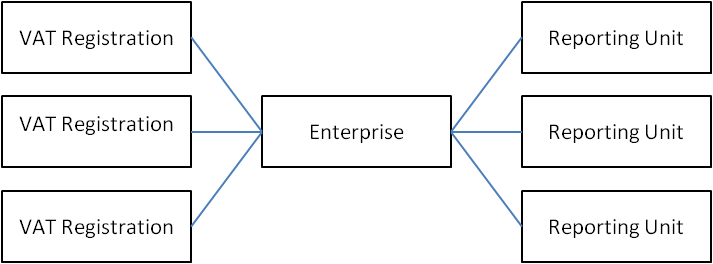
Summary
VAT turnover data has great potential to increase the number of businesses represented by our main measures of economic growth. As the brief analyses in this section demonstrate, the VAT turnover covers a vast number of typically smaller businesses.
We continue to develop statistical methods to make the best use of the data, in particular addressing the timeliness of the returns and the apportionment of the data to appropriate statistical units.
The next research article on the development of the VAT turnover data will be published in May 2017. It will include an update on the latest progress of the VAT project and provide results of analysis of the VAT turnover dataset on the new statistical processing platform.
References
Allcoat, J (2015) “Feasibility study into the use of HMRC turnover data within Short-term Output Indicators and National Accounts” Office for National Statistics
Stephens, M and Allcoat, J (2015) “Exploitation of HMRC VAT data” Office for National Statistics
Stephens, M and Allcoat, J (2015) “HMRC VAT update December 2015” Office for National Statistics
Allcoat, J (2016) “HMRC VAT update April 2016” Office for National Statistics
Stephens, M, Allcoat, J and Brown, B (2016) “VAT update July 2016” Office for National Statistics
Stephens, M, Allcoat, J and Brown, B (2016) “VAT Turnover, initial research analysis, UK: Jan 2014 to Mar 2016” Office for National Statistics
Edwards, L, Stephens, M, Allcoat, J, Painter, A, Rice–Mundy, G (Feb 2017) “VAT turnover, research analysis, UK: Jan 2014 to June 2016” Office for National Statistics
Notes for: Transforming turnover using VAT turnover data in the national accounts
The Monthly Business Survey samples Reporting Units selected from the Inter-Departmental Business Register.
An enterprise is an organisational unit producing goods or services which has a certain degree of autonomy in decision-making. An enterprise can carry out more than one economic activity and it can be situated at more than one location. An enterprise may consist out of one or more reporting units.
6. Improvements to early estimates of GDP through the 2008 to 2009 downturn
Introduction
Estimating gross domestic product (GDP) when economical activity is volatile is, naturally, more difficult than during a period of sustained steady economic growth. The economic downturn of 2008 to 2009 proved particularly difficult to estimate and we have faced some criticism that the turning points in the economic cycle were not identified quickly enough.
In particular the National Statistics Quality Review of National Accounts and Balance of Payments (Barker and Ridgeway 2014) made a recommendation that:
“….. the ONS undertake a thorough study of the 2008 to 2009 economic cycle and how the three measures of GDP and the short-term indicators performed in measuring quarterly economic growth. This study should look at how the current quarterly and annual processes and procedures contributed to the larger than normal revisions for this period with a view to possible changes that might improve the performance during future economic cycles”.
This analysis looks at how the initial published GDP estimates have subsequently been revised over the following quarters and years using the size of the overall revision through time as the main measure. Sometimes the magnitude of revision will also change the sign of the growth estimate from positive to negative (or the other way around) and cause turning points in the economy to change quarters. We suggest some reasons for the revisions at various vintages of GDP and we look at what improvements could be made to the estimation process to better predict turning points in the economy. Many of the improvements discussed in this analysis have already been implemented into the GDP quarterly rounds published since summer 2016.
Initial vintages of GDP
This analysis assumes a basic knowledge of the GDP process, especially regarding the initial short-term estimates versus the annual benchmarks in the December Quarterly National Accounts round and then on to the annual Supply and Use balanced datasets, but for those not familiar with the process further information can be found in A short guide to the UK National Accounts. Unless otherwise stated all data in this analysis are seasonally adjusted estimates and have had the effect of price changes removed (in other words, the data are deflated to provide volume estimates), with the exception of income data that are only available in current prices.
The primary interest in this article is around whether turning points in the economy could have been identified more quickly, rather than a detailed look at the exact length or depth of the economic downturn of 2008 to 2009. With this in mind it is a useful reminder to initially review the quarterly growth estimates as they were first published before the economic downturn occurred.
The economy had been slowing from the middle of 2007, as these various vintages of Quarter 2 (Apr to June) 2007 to Quarter 1 (Jan to Mar) 2008 GDP show. Figure 6 shows that the initial positive 0.4% estimate of Quarter 1 2008 GDP growth at the preliminary GDP publication was subsequently revised down to positive 0.3% and this is below the average seen over the preceding years.
Figure 6: Quarterly GDP growth slows before the economic downturn
Quarter 2 (Apr to June) 2007 to Quarter 1 (Jan to Mar) 2008, UK
Source: Office for National Statistics
Notes:
- Q1 refers to Quarter 1 (Jan to Mar), Q2 refers to Quarter 2 (Apr to June), Q3 refers to Quarter 3 (July to Sept) and Q4 refers to Quarter 4 (Oct to Dec).
Download this chart Figure 6: Quarterly GDP growth slows before the economic downturn
Image .csv .xlsIt is particularly noticeable that the June 2008 vintage of GDP introduced downward revisions across most of this period. June 2008 was not a Blue Book dataset, so these revisions were part of the regular quarterly round. The widespread downgrading of GDP growth was primarily due to the business and finance element of the Index of Services for Output.
Within expenditure, the downward revisions were from government final consumption expenditure (Quarters 2 and 3 2007), gross fixed capital formation (Quarter 2 2007), inventories (Quarter 4 2007 and Quarter 1 2008) and imports were generally revised up quite strongly, which also serves to reduce GDP growth. So most elements of expenditure turned out to be weaker than first estimated as more data were received.
Focus on Quarter 2 2008
Against this backdrop of a slowing economy, the main quarter in terms of identifying the turning point in the economy was Quarter 2 (Apr to June) 2008 and this section looks at that quarter in depth.
The preliminary GDP estimate for growth in Quarter 2 2008 was positive 0.2% but this was then revised down to 0.0% growth by the time of the September Quarterly National Accounts 2 months later as shown in Figure 7.
Figure 7: The profile of quarter-on-quarter GDP growth up to Quarter 2 (Apr to June) 2008 at September 2008 quarterly national accounts
UK
Source: Office for National Statistics
Download this chart Figure 7: The profile of quarter-on-quarter GDP growth up to Quarter 2 (Apr to June) 2008 at September 2008 quarterly national accounts
Image .csv .xlsThe preliminary estimate of positive 0.2% for GDP growth was driven by the Index of Services (IoS) that had growth of positive 0.4%. Within the IoS, adjustments are applied to improve the profile of the low level detailed series. Normally these are broadly offsetting at the top level of IoS, however, in this preliminary estimate the net impact of adjustments was to remove 0.38 percentage points from Quarter 2 GDP growth – or in other words, without adjustments the initial estimate of Quarter 2 2008 GDP growth would have been much stronger at 0.6%.
Adjustments may be applied when either there are unexplained or unverified movements in the turnover data received by the Monthly Business Survey, or if there are forecast series that look implausible. For the preliminary estimate the third month of the quarter contains a larger element of forecast data.
In this particular instance, some of the adjustments would have been required to correct the Arima forecasts for the month of June, which may have been weaker than expected if the April and May Monthly Business Survey returns were coming in lower than anticipated. In this quarter the initial data and forecasts were coming in far stronger than we were expecting based on other evidence in the public domain, so downward adjustments were applied. Even so the Bank of England commented in their August 2008 inflation report that the initial positive 0.2% growth in GDP was “a bit strong – expecting tough times for output”.
The Index of Production (IoP) estimates within preliminary GDP were for a month-on-month fall of 0.5% for the period of June 2008 and quarter-on-quarter growth for Quarter 2 in IoP of negative 0.8%. At the time this fall in IoP was challenged internally as part of the quality assurance process – external evidence was used to support the movement including comments from the British Chamber of Commerce report, which highlighted “serious risks of recession” as most manufacturing balances declined sharply. The Chartered Institute of Procurement and Supply saw their headline indicator of economic activity fall from 49.5 in May to 45.8 in June (any figure below 50 signifies contraction).
Figure 7 shows that by the time of the Second Estimate of GDP Quarter 2, growth was only just above 0.0% – by this time some expenditure information had been included. Gross fixed capital formation showed a quarter-on-quarter fall of 5.3% and within this business investment decreased by 4.7%, which again was consistent with the picture being presented by sources external to us. This weaker position was then confirmed in the full Quarterly National Accounts dataset for Quarter 2 2008 when GDP growth stood at 0.0%.
Around the same time as the Quarter 2 2008 Quarterly National Accounts some other major economic stories corroborated the marked slowdown in GDP:
the Bank of England produced their GDP projection graph as part of the quarterly inflation report, and this showed that forecasts for Quarter 3 (July to Sept) and Quarter 4 (Oct to Dec) 2008 predicted that GDP growth was almost as likely to be negative as it was to be positive
the International Monetary Fund (IMF) downgraded their growth forecasts for both 2008 and 2009
the European Union group of 15 countries (EU15) showed a negative GDP figure for Quarter 2 2008
Throughout the remaining vintages right through to June 2009’s Blue Book dataset, the estimate for Quarter 2 2008 remained at 0.0%, although it is interesting to note that rather than adjustments to the IoS taking 0.4 percentage points off GDP as they had done initially, they were now adding 0.1 percentage points to GDP, so there had been some weakening as forecasts were replaced by detailed level turnover data. For the next four quarterly GDP rounds the Quarter 2 growth estimate only weakened very slightly to negative 0.1% and remained there until the first annual supply and use balance of 2008 in Blue Book 2010.
Impact of re-profiling quarterly data when annuals are revised
This section continues to focus still on the revisions to Quarter 2 (April to June) 2008. Whereas the previous section discussed all the quarterly national accounts updates, in this section all the quarterly updates have been completed and we are now into the annual supply and use process, referred to usually as Blue Book.
At the Blue Book stage, further data sources are introduced and the three approaches to measuring GDP (production, income and expenditure) are fully balanced in current prices. When the annual balance is produced in current price terms this is then deflated (for expenditure and output) and a chained volume measure (CVM) quarterly path is then produced within the constraints of the annual total. In some respects this is quite a mechanical and mathematical process so it is not always possible to profile the exact quarterly path that we might like within the annual constraints.
This has been a particular issue with the quarters of 2008 where, at some Blue Books, we have not been able to reflect a strong enough first quarter (January to March) and a weak enough Quarter 4 (October to December) within the constraints of a strong positive 2007 annual growth and such a weak 2008 growth pattern.
The first Blue Book that impacted on the 2008 annual estimate was Blue Book 2010, which was a July Blue Book (Blue Books can be either published in July consistent with the June Quarterly National Accounts or published in October consistent with the September Quarterly National Accounts). It is worth saying that when the Blue Book is in July we don’t always have all the data sources in time for balancing, especially those that come from Her Majesty’s Revenue and Customs (HMRC) so it is often the following Blue Book when the full annual data sources are included.
Figure 8 shows the growth rate of Quarter 2 2008 at Blue Books 2009, 2010, 2011, 2012 and the latest position at Blue Book 2016. As Blue Book 2010 was a June Blue Book there was very little new information. As a result the growth rate of Quarter 2 2008 was revised from negative 0.1% to negative 0.3%.
Blue Book 2011 was the first true supply and use balance of 2008 with full data sources and the gross operating surplus element from HMRC came in much weaker than the quarterly sources and forecasts had been suggesting. Also, although annual compensation of employees was almost unchanged, there was a re-profiling of the quarters, which also made Quarter 2 2008 weaker. In hindsight, the Blue Book 2011 dataset showing negative 1.3% growth for Quarter 2 2008 and the quarterly path through the annual data points more generally were poor estimates.
This was rectified at Blue Book 2012 when the quarterly path was reassessed. Subsequent Blue Books have included the move to the European System of Accounts 2010 and taking on financial year data but we have remained broadly similar to that Blue Book 2012 position with growth of negative 0.7% for Quarter 2 2008 when we published Blue Book 2016.
Figure 8: Quarter on quarter growth rates of GDP at various Blue Books
UK, Quarter 2 (Apr to June) to Quarter 2 (Apr to June) 2008
Source: Office for National Statistics
Download this chart Figure 8: Quarter on quarter growth rates of GDP at various Blue Books
Image .csv .xlsSubsequent quarters in the economic downturn and recovery
The other quarters of the downturn and recovery can be reviewed in similar detail but, as the quarters within a calendar year are often affected in the same direction by the annual supply and use balance of a year, Table 2 is used to show the various vintages of GDP quarter-on-quarter growth for each period. Table 2 is read down the columns, so for instance the first data column is the Quarter 2 (Apr to June) 2008 dataset we have already presented. This shows the preliminary estimate of positive 0.2% in the first row, through the various vintages to the latest estimate in the last row.
Table 2: Quarter-on-quarter GDP growth at various vintages, UK, 2008 and 2009
| 2008 | 2009 | ||||||
| Quarter 2 | Quarter 3 | Quarter 4 | Quarter 1 | Quarter 2 | Quarter 3 | Quarter 4 | |
| Preliminary GDP | 0.2% | -0.5% | -1.5% | -1.9% | -0.8% | -0.4% | 0.1% |
| Quarterly national accounts | 0.0% | -0.6% | -1.6% | -2.4% | -0.6% | -0.2% | 0.4% |
| Last quarter before Blue Book 1 | -0.1% | -0.9% | -1.8% | -2.2% | -0.8% | -0.3% | 0.5% |
| Blue Book first balance | -0.3% | -0.9% | -2.1% | -1.6% | -0.2% | 0.2% | 0.7% |
| Blue Book second balance | -1.3% | -2.0% | -2.3% | -1.5% | -0.2% | 0.4% | 0.4% |
| Latest | -0.7% | -1.7% | -2.3% | -1.6% | -0.2% | 0.1% | 0.4% |
| Source: Office for National Statistics | |||||||
| Notes: | |||||||
| 1. Q1 refers to Quarter 1 (Jan to Mar), Q2 refers to Quarter 2 (Apr to June), Q3 refers to Quarter 3 (July to Sept) and Q4 refers to Quarter 4 (Oct to Dec). | |||||||
Download this table Table 2: Quarter-on-quarter GDP growth at various vintages, UK, 2008 and 2009
.xls (27.6 kB)Quarter 3 (July to Sept) 2008 was initially published at negative 0.5% and the regular quarterly updates weakened this figure to negative 0.9%. But it was the second Blue Book balance, in this case, Blue Book 2011, which gave us the much larger fall as information on gross operating surplus came in from HMRC.
Quarter 4 (Oct to Dec) 2008 has gradually weakened over the vintages from negative 1.5% initially to negative 2.3% now and has become the weakest quarter in the economic downturn. Quarter 1 (Jan to Mar) 2009 saw the biggest revision in quite a while between the preliminary estimate and the quarterly national accounts estimate 2 months later, with a revision of 0.5 percentage points, although since then this has been revised back the other way as slightly stronger data for 2009 were received in the annual process. As the economy started to pick up again in 2009 so the forecasts and early data lagged behind the pace of recovery indicated by later data subsequently received.
For Quarter 2 2009, the initial estimate of negative 0.8% was unchanged by the time of the last quarterly updates, but the first supply and use balance in Blue Book 2011 moved this figure up to negative 0.2% where it still is today. Initially it was thought that Quarter 3 2009 was also negative, but again the stronger data of Blue Book 2011 meant that this quarter turned to positive by the time of the first annual supply and use balance, shortening the downturn by 1 quarter.
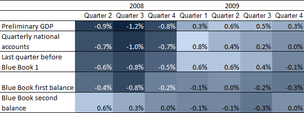
Table 3 is a heat map showing the difference between the estimate as it was published at the time and what the figure is today. The darker colouring signifies that the initial estimate has subsequently been revised down and the lighter colouring shows that the figure has since been revised up.
Table 3: Heat map of revisions to 2008 and 2009 quarterly GDP growth compared with the latest estimate
UK
Source: Office for National Statistics
Notes:
- Q1 refers to Quarter 1 (Jan to Mar), Q2 refers to Quarter 2 (Apr to June), Q3 refers to Quarter 3 (July to Sept) and Q4 refers to Quarter 4 (Oct to Dec).
Download this image Table 3: Heat map of revisions to 2008 and 2009 quarterly GDP growth compared with the latest estimate
.png (20.9 kB) .xls (29.7 kB)
What can clearly be seen from Table 3 is a distinct divide between 2008 on the left and 2009 on the right. 2008 has a lot of darker colouring, showing that as we entered the economic downturn our tendency was to revise our initial estimates to make them weaker.
Whereas in 2009 the lighter colouring shows that our initial estimates tended to be too weak and were revised up. Part of this is to do with the forecasting models we use, which are based on previous data in the time series and so tend to predict growth in the same direction as historic trends. Another reason for this could be the Monthly Business Survey and it is possible that businesses that are struggling to survive during the downturn are less likely to complete their survey returns on time. Similarly during the recovery phase the businesses that are performing best might be the slowest to return forms.
Lessons learnt and improvements made
Clearly the initial estimates of GDP growth going into the economic downturn of 2008 tended to over-estimate GDP and were subsequently revised down when fuller information was received from annual data sources. Likewise, the initial estimates of GDP growth in 2009 as the UK economy recovered tended to under-estimate the position and were later revised up. We have looked in detail at the existing process, most of which is still the same as in 2008, to see what improvements could be made to produce more accurate initial estimates during the next economic downturn. The following are the main conclusions from our analysis and the actions we are taking, or indeed have already taken, as a result.
Forecasts (for data that were not yet available) struggled to pick up turning points (both negative and positive) and therefore in future we should not be afraid to bring other intelligence and expertise more fully into play. As a result we reviewed the specifications of the forecasting files ahead of the preliminary estimate of GDP in October 2016 to ensure they were all as optimal as possible. We also now use a Monthly Business Survey (MBS)-only estimate for internal quality assurance, which strips out all the forecast series so that we can compare the growth rate from genuine returned data with the growth rate obtained from the forecasted elements. A bias adjustment is also built into some areas of the accounts such as construction output, to reflect the fact that the businesses that are performing best are less likely to return their monthly survey early.
Although we did look at some external data and reports for supporting evidence at the time, we could have done a lot more. Now we hold explicit “curiosity” meetings to ensure that our figures face internal scrutiny and are challenged for coherence, consistency and credibility. We are also using Value Added Tax (VAT) data as a quality assurance tool to validate movements we are seeing in our MBS returns and to fine-tune forecasts. The VAT data has a much larger sample size than the MBS and later this year it will start to be used directly in some of our GDP estimates.
Focusing on just the chained volume measure estimate can mask movements in current price data and the deflators, which could be offsetting each other to a degree, especially in times of high inflation. We now look first at the current price data in more detail and consider the impact that we should be seeing based on the deflators. If the current price data are strong but the chained volume measure is behaving very differently because of the deflator then we review more closely whether this is telling us a coherent message or whether quality adjustments are required.
The adjustments applied to the Index of Services (IoS) at the lowest levels of detail were mainly in one direction and had an undue influence on top level GDP. We now look a lot more closely at the top level impact of the adjustments being made. Generally, since the analysis work for this article concluded, the amount of adjustment has been a lot smaller and the overall impact on quarterly GDP growth has been no greater than plus or minus 0.1 percentage points.
The business and finance sector of the Index of Services (IoS) was one area that was revised down after the preliminary estimate for Quarter 2 2008. We have worked with the Bank of England, who provide the majority of the finance data later on in the GDP process, for advice on forecasting in the financial services and insurance industries to ensure the optimum approach is taken.
Even when the annual picture was little changed we still ended up with large revisions to the quarterly path. A lot more attention is now paid to the quarterly path, especially where an annual figure is relatively unchanged. We also have quarterly information now to help us to apportion financial year data into the correct calendar years more optimally.
While all of these improvements will help us to identify more quickly turning points in the economy, it must be remembered that the early estimates of GDP are just that – estimates, and they are subject to uncertainty and a variance around the central estimate. Revisions will inevitability still occur and revisions should not necessarily be seen as a bad thing – often they are the consequence of a trade-off between quick initial estimates and subsequent revisions. We will continue to study our revisions performance as one measure of the quality of our estimates, including how UK GDP revisions compare with those of other countries and we will also look to make further improvements to the estimation process and data content as opportunities arise.
Nôl i'r tabl cynnwys7. Understanding the UK economy
This section of the Review provides an overview of the performance of the UK economy using data published by the Office for National Statistics (ONS) over the last 3 months.
GDP growth
Quarterly National Accounts, released on 31 March 2017, show that the UK economy grew by 0.7% in Quarter 4 (Oct to Dec) 2016, unrevised from the second estimate. There was a slight downward revision to quarter-on-quarter gross domestic product (GDP) growth in Quarter 3 (July to Sept) 2016 to 0.5%, however, economic growth in recent quarters remains broadly similar to the previously published growth path.
On a calendar year basis, the latest data show that GDP grew by 1.8% in 2016, unrevised from the second estimate of GDP. This is lower than the 2.2% growth seen in 2015 and also lower than the average rate of calendar year GDP growth in the decade prior to the downturn (2.9%).
International comparisons of GDP growth
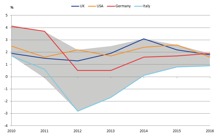
Figure 9 shows a range of growth rates for the G7 economies between 2010 and 2016. Germany saw the strongest annual GDP growth for 2016 at 1.9% outpacing the corresponding figures for the UK and the US (1.8% and 1.6% respectively). Italy has consistently the lowest rate of GDP growth of the G7 countries over this time period.
In 2016, the German economy expanded at its fastest rate in 5 years. This growth was largely driven by increases in employment and rising wages. Unemployment is at a record low and the numbers of people in work are at their highest level since reunification in 1990. Private consumption rose by 2.4% while public consumption increased by 4.2% boosted largely by refugee expenditure. Exports in Germany also performed strongly, rising by 2.5% year-on-year.
The United States recorded its slowest level of growth in 5 years, down from 2.6% in 2015. The strength of the dollar may have negatively affected exports, with poor trade performance accounting for most of the year-on-year decline in US GDP growth in the final 3 months of 2016.
UK growth stood at 1.8% in 2016, a slight decrease from the figure for 2015 (2.2%). Growth was driven predominantly by the services sector and household spending.
Figure 9: GDP chained volume measure
UK, USA, Germany, Italy and range of G7 countries, 2010 to 2016
Source: Organisation for Economic Co-operation and Development, Office for National Statistics
Download this image Figure 9: GDP chained volume measure
.png (19.0 kB) .xls (18.9 kB)
Productivity has grown 0.4% in Quarter 4 2016
Productivity – as measured by output per hour worked – increased by 0.4% in Quarter 4 (Oct to Dec) 2016, following growth of 0.2%, 0.3% and 0.3% in the 3 preceding quarters. As a result, labour productivity was around 1.2% higher in Quarter 4 2016 than in the same period a year earlier and grew consistently over 2016. A more detailed report on labour productivity estimates for the whole economy and a range of industries is available in our quarterly labour productivity bulletin.
When comparing the UK’s labour productivity with other economies, the UK ranks as the fifth most productive economy in the G7 in terms of output per hour and is approximately 16% less productive than the average for the rest of the G7. More details of these results can be found in the International Comparisons of Productivity release.
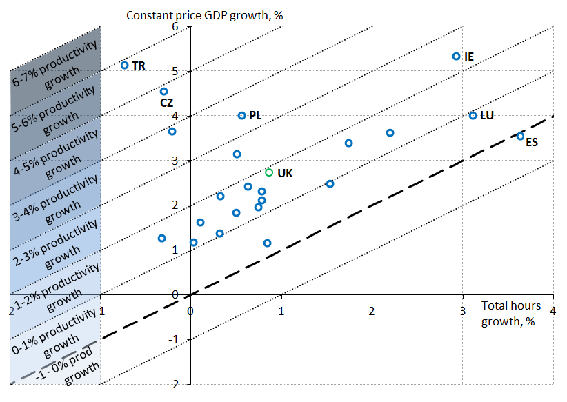
The relative weakness of recent labour productivity growth is one of the “puzzles” that define the UK’s productivity performance since the economic downturn. In order to understand this in a wider international context, Figures 10A and 10B present information on the compound average annual growth rates of GDP, hours and thus productivity for selected OECD economies over two periods: the 7 years prior to 2007 (Panel A) and between 2007 and 2015 (Panel B). Total hours growth is shown on the horizontal axis, GDP growth is shown on the vertical axis and the diagonal lines indicate combinations of hours and GDP growth consistent with varying degrees of productivity growth.
Figure 10a: Average GDP growth vs average total hours growth in OECD countries
Panel A: 2000 to 2007
Source: Organisation for Economic Co-operation and Development, Office for National Statistics
Notes:
- The country labels in Figures 10A and 10B use the standard International Organisation for Standardisation (ISO) 3166 country codes. The labelled countries are TR - Turkey, CZ - Czech Republic, PL - Poland, IE - Ireland, LU - Luxembourg, ES - Spain, and UK - United Kingdom.
Download this image Figure 10a: Average GDP growth vs average total hours growth in OECD countries
.png (94.8 kB) .xls (27.1 kB)
Figure 10b: Average GDP growth vs average total hours growth in OECD countries
Panel B: 2007 to 2015

Source: Organisation for Economic Co-operation and Development, Office for National Statistics
Notes:
- The country labels in Figures 10A and 10B use the standard International Organisation for Standardisation (ISO) 3166 country codes. The labelled countries are TR - Turkey, CZ - Czech Republic, PL - Poland, IE - Ireland, LU - Luxembourg, ES - Spain, and UK - United Kingdom.
Download this image Figure 10b: Average GDP growth vs average total hours growth in OECD countries
.png (95.4 kB) .xls (19.5 kB)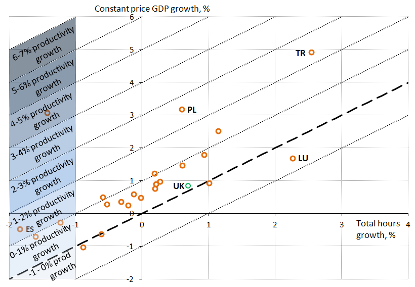
Panel A shows that during the pre-downturn period, average productivity growth was around 2% per year. In most cases this was achieved through stronger growth in GDP than the mostly positive growth in hours, however, the countries with the highest productivity growth were those that combined strong GDP growth with a fall in total hours. Only one nation – Spain – experienced negative productivity growth on average over this period.
Since the economic downturn – as shown in Panel B – rates of productivity growth fell markedly across these OECD nations, with average productivity growth falling to around 1% per year, while the UK’s productivity remained relatively unchanged. Panel B also provides some evidence that this weakening of labour productivity growth reflects a marked weakening of both GDP and total hours growth. Spain is again notable in this regard: having achieved positive productivity growth through a combination of falling hours worked and more modest falls in output. This data suggests that while the productivity puzzle may be particularly acute in the UK, weaker productivity growth since the recent downturn is not a phenomenon unique to the UK. More analysis on the UK’s productivity performance is available in our productivity introduction.
Consumption expenditure and growth of household debt is supporting services output growth
Figure 11 shows the performance of a composite industrial indicator based on output in “consumer-focused” industries. It shows that up until 2016, the consumer-focused industries perform broadly in line with growth in household loan liabilities (excluding lending secured on dwellings). The relationship with average wage growth, adjusted for inflation using the Consumer Prices Index (CPI), is also shown in Figure 11. CPI has been used, as at the time of the most recent labour market release, CPIH was not our headline measure of inflation. Since 21 March 2017, the Consumer Prices Index including owner occupiers’ housing costs (CPIH) has become our headline measure of inflation. Consequently CPIH will be used to estimate real earnings from next month’s labour market release.
Growth in real wages has moderated since late 2015, while consumer-focused services output has continued to grow strongly. With consumption continuing to grow strongly and real wage growth slowing, this has coincided with faster growth of loan liabilities. This increase in loan liabilities is having an impact on the household debt (excluding secured on dwellings) to income ratio (Figure 12). By the end of 2016, this ratio had almost returned to the 2008 average.
Figure 11: 12-month growth real wages, consumer-focused services and household loan liabilities (excluding secured on dwellings)
Quarter 1 (Jan to Mar) 2013 to Quarter 4 (Oct to Dec) 2016, UK
Source: Office for National Statistics
Notes:
“Consumer-focused services” include retail trade (45 and 47), food and beverage services (56), motion picture, TV and music activities (59), cultural activities, libraries and museums (91), gambling (92), and sports, amusement and recreation activities (93).
Q1 refers to Quarter 1 (Jan to Mar), Q2 refers to Quarter 2 (Apr to June), Q3 refers to Quarter 3 (July to Sept) and Q4 refers to Quarter 4 (Oct to Dec).
Download this chart Figure 11: 12-month growth real wages, consumer-focused services and household loan liabilities (excluding secured on dwellings)
Image .csv .xls
Figure 12: Household debt (excluding secured on dwellings) to income ratio
Quarter 1 (Jan to Mar) 2002 to Quarter 4 (Oct to Dec) 2016, UK
Source: Office for National Statistics
Notes:
Household debt includes all household and non-profit institutions serving households’ loan liabilities apart from loans secured on dwellings.
Q1 refers to Quarter 1 (Jan to Mar), Q2 refers to Quarter 2 (Apr to June), Q3 refers to Quarter 3 (July to Sept) and Q4 refers to Quarter 4 (Oct to Dec).
Download this chart Figure 12: Household debt (excluding secured on dwellings) to income ratio
Image .csv .xlsThe UK current account deficit reduces in Quarter 4 2016
The UK’s current account deficit as a percentage of GDP narrowed by 2.9 percentage points in Quarter 4 (October to December) 2016 to 2.4%. Figure 13 shows that the narrowing in the current account deficit was mainly due to a significant narrowing in the trade deficit and in the primary income deficit. The latter can be partially attributed to an increase in earnings, measured in sterling, on direct investments abroad, resulting in the smallest primary income deficit as a percentage of GDP seen since mid-2013.
Figure 13: The UK current account balance as a percentage of GDP
Quarter 1 (Jan to Mar) 2006 to Quarter 4 (Oct to Dec) 2016
Source: Office for National Statistics
Download this chart Figure 13: The UK current account balance as a percentage of GDP
Image .csv .xlsThe overall trade balance as a percentage of GDP narrowed by 2 percentage points in Quarter 4 2016 compared with the previous quarter - largely driven by an £7.6 billion increase in goods exports. Of this £7.6 billion, £2.5 billion can be attributed to increases in exports of erratic commodities (e.g. non-monetary gold, aircraft), with a further £1.6 billion attributed to exports of oil. Of the additional £3.5 increase in exports other than erratic and oil series, there was a large increase to the exports of machinery (£1.0 billion).
The overall narrowing in the UK’s current account deficit also coincided with a substantial depreciation in the sterling effective exchange rate, falling 17.0% between Quarter 4 2015 and Quarter 4 2016. Further information on the impact of a sterling devaluation on the Balance of Payments and International Investment Position can be found in the latest bulletin.
Exports of transport goods are helping to reduce the trade deficit
Between the 3 months to October 2016 and the 3 months to January 2017, the total trade deficit (goods and services) narrowed by £4.7 billion to £6.4 billion (Figure 14). These data also show a continuing surplus in total trade in services and total trade in goods deficits for both EU and non-EU countries. New data for trade, construction and production data covering February 2017 will be released on 7 April.
The main contributors to the narrowing of the deficit were increased exports of non-monetary gold, oil, machinery and transport equipment, and chemicals. In 2016, the UK’s largest exported commodity was mechanical machinery, with motor vehicles coming in as second highest. These trade figures corroborate the recent strength seen in UK manufacturing production – in the 3 months to January 2017, manufacturing output grew by 2.1% compared with the previous 3 months, the highest rate since May 2010.
Figure 14: Trade balance
Balance of payments basis, seasonally adjusted, UK, January 2015 to January 2017
Source: Office for National Statistics
Download this chart Figure 14: Trade balance
Image .csv .xlsMovements in sterling continue to have an impact on trade prices, with recent sterling depreciation coinciding with upward price pressure on both export and import prices. Goods import and export prices have risen 2.2% and 1.3% respectively in the 3 months to January compared with the 3 months to October 2016. While sterling appreciated slightly against a basket of currencies during this period (0.1%), it still remains 15.2% lower compared with the same period a year earlier (3 months to January 2016).
There is relatively strong 3-month on 3-month growth in infrastructure and housing repairs within overall construction output growth of 1.8%
Despite a 0.4% fall in construction output in January 2017, output grew by 1.8% on a 3-month on 3-month basis following consecutive rises in November and December (up 0.8% and 1.8% respectively). In particular, infrastructure, and private housing repairs and maintenance continue to show strong 3-month on 3-month growth, increasing at rates of 4.0% and 5.4% respectively. Only private industrial work and non-housing repair and maintenance experienced negative growth over the same period.
Total construction new orders fell by 2.8% in Quarter 4 (Oct to Dec) 2016, reflecting a fall in all sectors except for public work. Despite the quarterly fall, the annual volume of new orders is now at its highest level since 2008.
An increase in consumer price inflation is slowing real wage growth
The 12-month growth rate for the Consumer Prices Index including owner occupiers’ housing costs (CPIH) increased to 2.3% in February 2017. This has increased from the 12-month rate of 0.6% for February 2016.
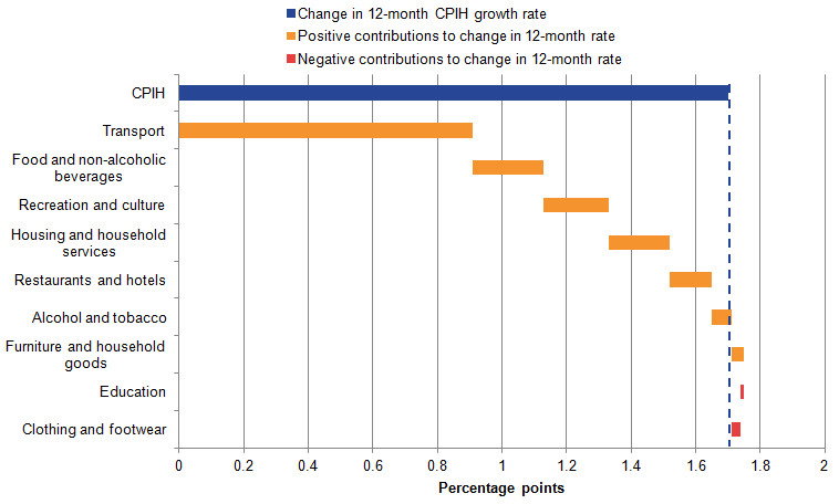
Figure 15 shows the main contributions to the change in the 12-month rate by each Classification of Individual Consumption According to Purpose (COICOP) division. The contribution from the transport division (0.9 percentage points) makes up the majority of the change in the CPIH 12-month rate (1.7 percentage points). Previous analysis showed that most of this change has come from the increase in the fuels and lubricants class, which has been affected by a combined effect of increases in the global crude oil price and the depreciation of sterling over this period.
Figure 15: Contributions to the change in the 12-month CPIH growth rate by COICOP division
UK, February 2016 to February 2017
Source: Office for National Statistics
Notes:
- The COICOP divisions for Health, Communication and Miscellaneous goods and services have been excluded from this chart, as they had a negligible effect on the change in the CPIH 12-month growth rate.
- Individual components may not sum due to rounding.
Download this image Figure 15: Contributions to the change in the 12-month CPIH growth rate by COICOP division
.png (17.7 kB) .xls (17.9 kB)
The increase in the CPIH 12-month rate can also be partly attributed to food and non-alcoholic beverages, which contributed around 0.2 percentage points to the overall change. Previous analysis (Prices economic commentary: Jan 2017) showed input producer prices for both domestically produced and imported food increasing in the second half of 2016, while output producer prices for food started to increase towards the end of 2016. In February 2017, the 12-month rate for food turned positive following almost 3 years of deflation.
Figure 16 shows rates of nominal and real wage growth over a 15-year period from January 2002. Wages have been adjusted for inflation using the Consumer Prices Index (CPI) as this series is available prior to 2005, whereas CPI including owner occupiers’ housing costs (CPIH) is available using the current methodology only from 2005. Consequently, we will be using CPIH (rather than CPI) to estimate real earnings from the next release resulting in revisions to estimates of real earnings. As the CPIH series currently commences in 2005 the estimates of real earnings will commence in 2005 from the next release.
These data show that regular weekly earnings for employees (excluding bonuses) in the UK increased by 2.3% in the 3 months to January 2017 compared with a year earlier. This is the weakest rate of growth since August 2016 and down from 2.6% in the 3 months to December 2016.
Once adjusted for inflation (measured by CPI) average weekly earnings increased by 0.8% in the 3 months to January 2017, excluding bonuses, compared with a year earlier. This is the weakest growth in real earnings since November 2014.
Figure 16: Regular average weekly earnings growth, seasonally adjusted, 3-month on 3-month a year ago: real and nominal
UK, January 2002 to January 2017
Source: Office for National Statistics
Notes:
- Dashed lines indicate pre-crisis averages (calculated over 2002 to 2007).
- Real wages are calculated using CPI rather than CPIH as a deflator as in Figure 11.
Download this chart Figure 16: Regular average weekly earnings growth, seasonally adjusted, 3-month on 3-month a year ago: real and nominal
Image .csv .xlsProvisional data shows minimal impact on GDP from changes being introduced in Blue Book 2017
As part of the communication plan for Blue Book 2017, we have published two articles this quarter that cover the impact that the improvements being introduced as part of Blue Book 2017 will have on GDP.
The first, on 16 February 2017 gave the impact on current price GDP estimates from 1997 to 2012; the second article, published on 13 March 2017 gave the impact on chained volume measure estimates of GDP from 1997 to 2012.
In summary, the range of current price changes being introduced in Blue Book 2017 have the combined impact of increasing the level of current price GDP in 2012 by approximately £10.2 billion, around 0.6%. Average annual current price GDP growth between 1997 and 2012 has been revised downwards by 0.1 percentage points from 4.0% per year to 3.9%.
Figure 17: Contributions to changes to current price GDP annual levels, near final impact
UK, 1997 to 2012
Source: Office for National Statistics
Notes:
- Dashed lines indicate pre-crisis averages (calculated over 2002 to 2007).
- Real wages are calculated using CPI rather than CPIH as a deflator as in Figure 11.
Download this chart Figure 17: Contributions to changes to current price GDP annual levels, near final impact
Image .csv .xlsThe main source of revision in Blue Book 2017 is from improvements to the methods used to estimate rental (both actual and imputed).
Most of the improvements to current price GDP in Blue Book 2017 directly impact on the estimates of real GDP as well. The package of real GDP changes as a whole, over the period 1998 to 2012, have the combined impact of very slightly reducing the average annual growth of real GDP by around 0.04 percentage points. However, the headline average over this period remains at 1.9% per year in Blue Book 2017, as it was in Blue Book 2016.
The average revision to quarter-on-quarter real GDP growth introduced at this Blue Book is negative 0.01 percentage points over the period from Quarter 2 (Apr to June) 1997 to Quarter 4 (Oct to Dec) 2012. Over the same period the absolute revision to quarter-on-quarter real GDP growth is 0.05 percentage points.
The peak to trough of the 2008 to 2009 economic downturn has been revised from negative 6.3% to negative 6.1%. As part of the March publication, we included an indicative quarterly path for real GDP (Figure 18), which shows that the Blue Book 2017 revisions do not change the economic narrative over this period.
Figure 18: Quarter-on-quarter growth in real GDP
UK, Quarter 2 (Apr to June) 1997 to Quarter 4 (Oct to Dec) 2012 for Blue Book 2016 and Blue Book 2017
Source: Office for National Statistics
Notes:
- These figures are still indicative at this stage and final quality assurance is currently being undertaken. A finalised version of these data will be provided in an updated article on 6 July 2017 which will include current price and chained volume measure GDP for 1997 to 2015, ahead of publication in the UK National Accounts on 29 September 2017.
- Q1 refers to Quarter 1 (Jan to Mar), Q2 refers to Quarter 2 (Apr to June), Q3 refers to Quarter 3 (July to Sept) and Q4 refers to Quarter 4 (Oct to Dec).
Download this chart Figure 18: Quarter-on-quarter growth in real GDP
Image .csv .xls8. Annex A – Publication dates and themes for future Economic reviews
Table A1 shows the provisional publication dates for the next three Economic reviews and their themes.
Table A1: Future publication dates for the Economic Review 2017 to 2018
| Publication date | Theme |
| 10 July 2017 | Impact on ONS data from changes in international factors such as oil prices, value of sterling |
| 19 October 2017 (provisional) | Labour market statistics development and analysis |
| 23 January 2018 (provisional) | Prices statistics development and analysis |
Download this table Table A1: Future publication dates for the Economic Review 2017 to 2018
.xls (26.1 kB)Economic Forum meetings will be held in London on the day of release of the Economic review.
Nôl i'r tabl cynnwys9. Annex B - Demand and supply indicators
Table 4: UK demand side indicators
| 2015 | 2016 | 2016 | 2016 | 2016 | 2016 | 2016 | 2016 | 2017 | 2017 | ||||
| Q2 | Q3 | Q4 | Oct | Nov | Dec | Jan | Feb | ||||||
| GDP | 2.2 | 1.8 | 0.6 | 0.5 | 0.7 | ||||||||
| Index of Services | |||||||||||||
| All Services1 | 2.6 | 2.9 | 0.6 | 0.9 | 0.8 | 0.3 | 0.2 | 0.2 | -0.1 | .. | |||
| Business Services & Finance1 | 2.9 | 2.4 | 0.7 | 0.7 | 0.5 | - | 0.4 | -0.1 | 0.5 | .. | |||
| Government & Other1 | 0.5 | 1.6 | 0.1 | 0.3 | 0.4 | - | 0.2 | 0.1 | 0.2 | .. | |||
| Distribution, Hotels & Rest1 | 4.5 | 5.1 | 0.9 | 1.1 | 2 | 1.3 | 0.2 | -0.4 | -0.7 | .. | |||
| Transport,Stor. & Comms1 | 3.7 | 3.7 | 0.6 | 2.6 | 1 | 0.1 | -0.4 | 2 | -1.2 | .. | |||
| Index of Production | |||||||||||||
| All Production1 | 1.2 | 1.2 | 2.2 | -0.4 | 0.3 | -1.2 | 2.3 | 0.9 | -0.4 | .. | |||
| Manufacturing1 | -0.2 | 0.7 | 1.8 | -0.7 | 1.2 | -1 | 1.4 | 2.2 | -0.9 | .. | |||
| Mining & Quarrying1 | 8.4 | 0.6 | 2.3 | 4.5 | -7 | -8.1 | 7.8 | -1.3 | 1.4 | .. | |||
| Construction1 | 4.9 | 2.4 | 0.9 | -0.3 | 1 | ||||||||
| Retail Sales Index | |||||||||||||
| All Retailing1 | 4.4 | 4.9 | 1 | 1.7 | 1.1 | 2.2 | -0.2 | -2.1 | -0.5 | 1.4 | |||
| All Retailing excl Fuel1 | 4 | 4.7 | 1.2 | 1.7 | 1.5 | 2.3 | 0.1 | -2.2 | -0.3 | 1.3 | |||
| Predom. Food Stores1 | 2.2 | 3.7 | 0.2 | 1.3 | 0.2 | 1.1 | -0.6 | -1.4 | -0.3 | 0.1 | |||
| Predom. Non-Food Stores1 | 4.3 | 3.5 | 1.2 | 1 | 1.3 | 3.1 | -0.2 | -2.4 | -0.3 | 1.8 | |||
| Non-Store Retailing1 | 13.1 | 16.7 | 6.1 | 7.1 | 8.1 | 3.6 | 4.1 | -4.4 | -0.9 | 4 | |||
| Trade | |||||||||||||
| Balance2 3 | -29.8 | -36 | -7.8 | -13.7 | -5 | -0.6 | -2.4 | -2 | -2 | .. | |||
| Exports4 | 1.1 | 5.2 | 4.7 | 0.6 | 6.6 | 5.1 | 1.8 | 1.5 | 0.8 | .. | |||
| Imports4 | -0.1 | 6.1 | 3 | 4.8 | 0.2 | -5 | 5.6 | 0.6 | 0.6 | .. | |||
| Public Sector Finances | |||||||||||||
| PSNB-ex5 | -22.6 | -22.2 | -3.6 | -4.6 | -6.9 | -2.7 | -2 | -2.2 | -2 | -2.8 | |||
| PSND-ex as a % GDP | 84.7 | 86 | 84.1 | 83.9 | 86 | 83.8 | 84.5 | 86 | 85 | 85.4 | |||
| Source: Office for National Statistics | |||||||||||||
| Notes: | |||||||||||||
| 1. Percentage change on previous period, seasonally adjusted, CVM | |||||||||||||
| 2. Levels, seasonally adjusted, CP | |||||||||||||
| 3. Expressed in £ billion | |||||||||||||
| 4. Percentage change on previous period, seasonally adjusted, CP | |||||||||||||
| 5. Public Sector net borrowing, excluding the impact of financial interventions. Level change on previous period a year ago, not seasonally adjusted | |||||||||||||
Download this table Table 4: UK demand side indicators
.xls (31.2 kB)
Table 5: Supply side indicators
| 2015 | 2016 | 2016 | 2016 | 2016 | 2016 | 2016 | 2016 | 2017 | 2017 | ||||
| Q2 | Q3 | Q4 | Oct | Nov | Dec | Jan | Feb | ||||||
| Labour Market | |||||||||||||
| Employment Rate1 2 | 73.7 | 74.4 | 74.5 | 74.5 | 74.6 | 74.5 | 74.6 | 74.6 | .. | .. | |||
| Unemployment Rate1 3 | 5.4 | 4.9 | 4.9 | 4.8 | 4.8 | 4.8 | 4.8 | 4.7 | .. | .. | |||
| Inactivity Rate1 4 | 22 | 21.7 | 21.6 | 21.7 | 21.6 | 21.7 | 21.6 | 21.6 | .. | .. | |||
| Claimant Count Rate7 | 2.3 | 2.2 | 2.2 | 2.3 | 2.3 | 2.3 | 2.3 | 2.3 | 2.2 | 2.1 | |||
| Total Weekly Earnings6 | 491 | 503 | 502 | 505 | 508 | 507 | 509 | 507 | 507 | .. | |||
| CPI | |||||||||||||
| All-item CPI5 | - | 0.7 | 0.4 | 0.7 | 1.2 | 0.9 | 1.2 | 1.6 | 1.8 | 2.3 | |||
| Transport5 | -2.1 | 0.5 | -0.9 | 0.8 | 2.8 | 2.3 | 2.5 | 3.7 | 5.7 | 6.9 | |||
| Recreation &Culture5 | -0.6 | 0.4 | 0.5 | 0.7 | 0.6 | 0.2 | 0.7 | 0.9 | 0.9 | 1.6 | |||
| Utilities5 | 0.5 | 0.2 | - | - | 0.3 | 0.3 | 0.2 | 0.4 | 0.6 | 0.7 | |||
| Food & Non-alcoh Bev5 | -2.6 | -2.4 | -2.7 | -2.3 | -1.8 | -2.4 | -2 | -1.1 | -0.5 | 0.2 | |||
| PPI | |||||||||||||
| Input8 | -12.8 | 2 | -4.1 | 6.5 | 14.1 | 12.4 | 13.5 | 16.6 | 20.1 | 19.1 | |||
| Output8 | -1.7 | 0.4 | -0.4 | 0.8 | 2.4 | 2.1 | 2.4 | 2.8 | 3.6 | 3.7 | |||
| HPI8 | 5.9 | 7.3 | 8.7 | 7.1 | 5.6 | 6.1 | 5.3 | 5.7 | 6.2 | .. | |||
| Source: Office for National Statistics | |||||||||||||
| Notes: | |||||||||||||
| 1. Monthly data shows a three month rolling average(e.g. The figure for November is for the three months ending in November) | |||||||||||||
| 2. Headline employment figure is the number of people aged 16-64 in employment divided by the total population 16 to 64 | |||||||||||||
| 3. Headline employment figure is the number of unemployed people (aged 16+) divided by the economically active population (aged 16+) | |||||||||||||
| 4. Headline inactivity figure is the number of economically active people aged 16-64 divided by the 16 to 64 population | |||||||||||||
| 5. Percentage change on previous period a year ago, seasonally adjusted | |||||||||||||
| 6. Estimates of total pay include bonuses but exclude arrears of pay (£) | |||||||||||||
| 7. Calculated by JSA claimants divided by claimant count plus workforce jobs | |||||||||||||
| 8. Percentage change on previous period a year ago, non-seasonally adjusted | |||||||||||||