1. Introduction
The National Statistician’s Data Analysis and Methods review in privacy and data confidentiality identified differential privacy as one of the potential tools the Office for National Statistics (ONS) could employ to provide more transparent and well-defined levels of protection to data. Reconstruction attacks by Dinur and Nissim have shown that traditional statistical disclosure control methods, such as record swapping might not provide sufficient protection to tabular data. Differentially private data are not vulnerable to reconstruction attacks, therefore differential private methods might prove essential to obtain respondents’ confidence in the statistical institute.
The ONS is firmly committed to applying cutting-edge statistical disclosure control methods to get respondents’ trust and keep survey response rates high. Exploring differential privacy and its applications must therefore be a significant part of the ONS disclosure control workplan in the coming years. The present paper explores how the ONS might implement simple differentially private methods to release frequency tables. Providing a broad outlook on differential privacy in the context of frequency tables is out of the scope of this paper.
The purest definition of differential privacy has a single parameter epsilon (ε) to indicate the level of protection, lower values of ε indicate more protection. Many methods can fulfil the definition, one of which is the addition of noise from a Laplace distribution. The Laplace mechanism perturbs frequencies to fractions and therefore some adjustment, for example rounding, needs to be applied to produce an output that is credible for users. Such adjustments preserve the differentially private property of the output since they can be considered post-processing (PDF, 2,081KB). This paper explores a relatively simple Laplace implementation, and identifies practical drawbacks. The geometric mechanism, and Gaussian mechanism, were also applied, though results are not presented here.
A differential privacy pilot was run on mortality data within the ONS secure environment. Outputs were produced using two different differential privacy approaches. The first approach was to directly add noise to frequency table counts, for a range of tables and ε values. This approach is similar to another post-tabular noise method, cell-key perturbation, with two major differences.
The first difference is the privacy budget. In the differential privacy paradigm, each output contributes to the overall disclosure risk. In practice often the overall ε for a given set of outputs is determined first; we call it the privacy budget. A fraction of the whole budget is then allocated to each output. For a total budget of ε and 10 frequency tables, for example, uniform allocation of the budget means applying a differentially private random mechanism with parameter ε/10 to each table. Non-uniform allocation of the privacy budget is also possible. Publications with a limited number of outputs, known ahead of time will be better suited to this kind of budgeting. Further releases of data increase the amount of budget used and weakens the privacy guarantee.
The second difference concerns the perturbation of zeros. To meet the differential privacy standard, zero cells need to be treated like all other cells. This might result in negative noise given to zero cells, and apparent negative cell counts. Post-processing can be used to ensure non-negativity of all cells, but a direct correction (for instance, rounding up negative cells to zero) will lead to a systematic bias. In cell key perturbation the noise applied depends on the cell value such that cells do not receive negative noise larger than their original value. Zeros are treated differently to other cells and do not receive negative noise.
The second, “top-down” method creates a set of microdata from post-noise frequency tables. The microdata as a whole is produced within the ε budget, so any number of outputs can be produced without exceeding a fixed budget. The idea of this approach follows the work the US Census Bureau have carried out for Census 2020, to protect against the risk of reconstruction attacks. Under differential privacy, zeros and small counts still need to be treated like other cells, which leads to a significant bias issue in our implementation. This approach may be impractical using a large number of variables. The process would become computationally intensive, though this constraint will likely ease in future with increased processing capacity. In a hypothetical scenario with more than 50 variables, considering such a level of detail would distinguish essentially every record as unique. A frequency table of this detail would consist of only zeros and ones (no or one person with this combination of characteristics) and it would be difficult for noise to affect the counts to provide protection without overpowering them entirely, especially if it is assumed the post-noise counts would need to be integers in which case the noise added to each cell would be minus 1, plus 1, or greater.
Nôl i'r tabl cynnwys2. Differential privacy
A randomised mechanism M is defined as providing ε differential privacy if for all datasets D, D’, which differ by only one record, for all S ⊆ range(M):
Between any two sets of data that differ by only one record, the ratio of probabilities of getting the same result is bounded by exp(ε). In other words, the data release process is nearly equally likely to get the same result, even if you add or remove one record from the original data. The definition encourages a member of the public to fill in and return their survey form. Under differential privacy, the act of returning the form is guaranteed to make nearly no difference to the statistics and results produced, while the collective survey results will still provide insight and value. The bound on the ratio is tightest with small ε values. Small values of ε (less than one) imply strong protection, larger values imply weaker protection. Practical uses of differential privacy, for example, the Disclosure Avoidance System of the US Census Bureau, an approach developed by Apple, or an example for protecting survey weighted frequency tables (PDF, 1,294KB), have had values between 1-8. The choice of ε is a policy decision.
Figure 1: Illustration of differential privacy definition - Laplace noise

Download this image Figure 1: Illustration of differential privacy definition - Laplace noise
.png (106.8 kB)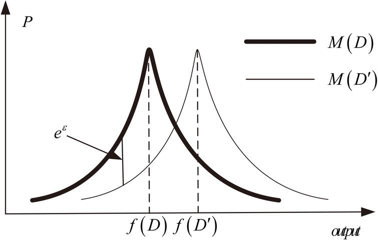
By virtue of the shape of Laplace noise, it can be shown that, for frequency tables, the ratio of P(M(D)) to P(M(D’)) is always less than exp(ε) where the noise produced is Laplace(1/ε), therefore meeting the definition. Reducing ε reduces the allowed relative distance between the two curves and increases the magnitude of noise (flattening the Laplace curves).
Differential privacy provides a strong guarantee of privacy that in its simplest form can be summarised in one parameter. It has also been described as a formal guarantee of privacy and referred to as a “formal privacy” method. It forms a worst-case scenario, assuming intruders hold large amounts of private knowledge and employ sophisticated attacks. Unlike in the case of traditional statistical disclosure control methods, releasing the parameter does not affect the level of protection, the release of ε values is strongly encouraged in the principle of transparency, and to help users evaluate and account for the impact the protection has on results.
Nôl i'r tabl cynnwys3. Comparing differential privacy with traditional disclosure control methods
Although the measurement of protection differs between differential privacy and traditional disclosure control, achieving differential privacy through post-tabular noise addition is very similar to other post-tabular perturbation methods including cell-key perturbation.
In this section we consider the impact of epsilon, and how the values would compare with a perturbation rate used in cell-key perturbation. We look at what proportion of cells in a single frequency table would receive (non-zero) noise in a differential privacy setting, using a range of epsilon values. For the Laplace and Gaussian mechanisms, we assume that rounding to the nearest integer is carried out after noise addition. A cell remains unchanged if the noise added to the cell (without rounding) is larger than (-0.5) and smaller than 0.5. If the noise variable is Y, and its cumulative distribution function (CDF) is F(y), the probability of zero noise is:
The cumulative distribution function of the Laplace(1/ε) distribution is
The probability of zero noise is
The probability of a cell being changed is
The following table summarises the probabilities for five different ε values.
| ε | 0.1 | 1 | 2 | 5 | 10 |
|---|---|---|---|---|---|
| 1 − exp (− ε/2) | 0.0488 | 0.3935 | 0.6321 | 0.9179 | 0.9933 |
| exp (− ε/2) | 0.9512 | 0.6065 | 0.3679 | 0.0821 | 0.0067 |
Download this table Table 1: Laplace noise probabilities
.xls .csvOn a single table with Laplace(1/ε) noise added, for ε = 0.1, an expected 4.9% of cells would remain unchanged. For ε=10, an expected 99.3% of cells would remain unchanged.
Equivalent probabilities can be calculated using the Gaussian and Geometric cumulative distribution functions:
| ε | 0.1 | 1 | 2 | 5 | 10 |
|---|---|---|---|---|---|
| P(cell value is unaltered) | 0.0157 | 0.1562 | 0.3065 | 0.6755 | 0.9512 |
| 1−P(cell value is unaltered) | 0.9843 | 0.8438 | 0.6935 | 0.3245 | 0.0488 |
Download this table Table 2: Gaussian noise probabilities
.xls .csv
| ε | 0.1 | 1 | 2 | 5 | 10 |
|---|---|---|---|---|---|
| P(cell value is unaltered) | 0.05 | 0.4621 | 0.7616 | 0.9866 | 0.9999 |
| 1−P(cell value is unaltered) | 0.95 | 0.5379 | 0.2384 | 0.0134 | 0.0001 |
Download this table Table 3: Geometric noise probabilities
.xls .csvThese calculations provide a broad idea of how much perturbation is involved using a range of epsilon values. These will not act as a direct equivalence, particularly considering the privacy budget when multiple outputs are produced, and the perturbation of zeros and small counts which are treated differently to other cells in cell-key perturbation.
Nôl i'r tabl cynnwys4. Differential privacy pilot
One of the recommendations of the National Statistician’s Data Analysis and Methods review on privacy and confidentiality was that the Office for National Statistics (ONS) should run a differential privacy pilot study, on low-sensitivity data. We have applied differential privacy protection to outputs on mortality data, within a secure environment. Mortality data was chosen as it covered a complete population rather than being a sample and contained a large enough population to produce a wide range of outputs without being burdensome to process. The microdata contained one record for each death registered in England and Wales in 2018, approximately 541,000 in total. Each record contained some demographic information of the deceased including age, sex, and area of residence, alongside information such as date and cause of death.
Method 1: “Independent noise addition”
Differential privacy is not a specific protection method, several methods can be shown to meet the definition of differential privacy, though the addition of Laplace noise is common. The simplest form which we refer to as “independent noise” method, is to produce frequency tables and add noise to the table counts. In a similar way to the cell-key perturbation method, totals will not be consistent between different tables and additivity will not be preserved between levels in a hierarchy if calculated independently. Post-processing could be applied within the differential privacy definition to re-establish consistency, additivity for such tables. There are many potential approaches to this post-processing and a simple implementation is the focus here. As well as Laplace, noise generated from a Gaussian and geometric mechanism can also be shown to fit the differentially private definition (PDF, 2,081KB).
Privacy budget
Frequency tables produced in this way individually meet the differential privacy standard and each have a value of epsilon. However, each release of a table is a separate source of data and adds to the total ε budget of the release (PDF, 470KB). If we decided on a budget of ε of 10 for a dataset, this would allow releasing of 10 tables each with use of ε of one, or 100 tables with ε of 0.1. To guarantee a budget of ε would not be exceeded, it would be necessary to have a fixed number of outputs.
Perturbation of zeros
The second issue with applying differential privacy is the way zeros need to be treated. Zeros need to be given noise in the same way as any other cell. Consider a respondent choosing whether or not to return their form. Assume that this respondent is unique so that if they return their survey the cell containing them would be a ‘1’. Not responding, this cell would be ‘0’. Without perturbation of zeros, the cell would certainly be ‘0’ under a non-response. The cell would never take a value of 1, 2… so the ratio of probabilities will be outside the range allowed by the definition.
If zeros are perturbed, larger tables at low geography may be heavily affected. Sparse tables at low geographies can contain mostly zero values, in which case the majority of noise is given to zero-cells. This is a helpful feature for reducing disclosure risk and introducing more uncertainty on small counts, but often carries a disproportionately high utility cost.
Negative values and bias
The other related issue is how to treat apparent negative values. When zero-cells or small counts receive noise, the result can be a negative value. In the purest form of differential privacy negative values would be released to the end user, but post-processing is possible within the differential privacy framework. Negative values could be rounded up to 0 without compromising the protection, however this would result in an overall positive bias that would need to be either reported or adjusted for elsewhere in the table, which, depending on the scale of the noise may be difficult to compensate for.
Method 2: “Top-down method”
A more sophisticated method can also be considered, which could be described as having parallels with synthetic data. The principle is that noise is added to a large table at national geography, then the values are disaggregated to lower levels (for example, national, regional, local).
To meet the differential privacy standard, noise needs to be added at every level of geography. This can also be thought of as adding noise to any data included in the process. This produces a set of constraints for each level of geography, which could be solved simultaneously or sequentially. The US Census Bureau intend to use a large optimisation program (PDF, 10,195KB) and match constraints at all geography hierarchy levels. Some structural zeros are imposed using some of the ε budget. Releasing analysis of how outputs from the differentially private data compare to outputs from the pre-protection data also expends some ε budget. A simpler method applied here matches constraints at the highest geographies first, then considers these to be fixed when producing lower levels. Details are shown in Figure 2.
Figure 2: Top-down method illustration

Source: Office for National Statistics
Download this image Figure 2: Top-down method illustration
.png (74.8 kB)
The top-down method aims to produce a differentially private microdata set (it could also be thought of as a large hypercube) where each cell has been influenced by differentially private noise (for example Laplace noise). The microdata set itself will be differentially private, so that an unlimited number of outputs could be produced without going over an ε privacy budget, and all outputs will be additive and consistent with each other.
Starting at “the top”, the highest aggregate of total population has noise added, and the count is rounded to a whole number. This is the new population total. Next, the frequency table of all variables is produced at national geography level (no geography breakdown). Noise is added to this table, and totals are adjusted to match the new total population size. Each value is multiplied by the new population size and divided by the total of post-noise values. This is analogous to disaggregating the total population into cells based on the post-noise national table.
Similarly, the table of all variables is split by a geography breakdown, noise is added, then adjusted to match the national level counts (and rounded to whole numbers). A table can be produced at a low level of geography, then adjusted to higher geography counts.
Note that the tables are additive to the upper level in the hierarchy after the adjustment but are not integer values. Basic rounding would often alter the totals and ruin the additivity, so a smarter form of rounding needs to be applied which preserves totals/sub-totals. A “maximum remainder method” was used, but alternatives are available.
| Table Number | Geography | Variables | ||
|---|---|---|---|---|
| 1 | Clinical Commission group (CCG) | Cause of death | Age | Sex |
| 2 | CCG | Cause of death | Month of death | Sex |
| 3 | CCG | Cause of death | Marital Status | Sex |
| 4 | CCG | Month of death | Age | |
| 5 | CCG | Month of death | Marital Status | |
| 6 | CCG | Cause of death | ||
| 7 | CCG | Age | ||
| 8 | CCG | Sex | ||
| 9 | CCG | Month of death | ||
| 10 | CCG | Marital Status | ||
| 11 | Region | Cause of death | Age | |
| 12 | Region | Cause of death | Month of death | |
| 13 | Region | Cause of death | Sex | |
| 14 | Region | Month of death | Sex | |
Download this table Table 4: Frequency tables produced in pilot
.xls .csvThese are the tables produced using independent noise and tabulated from the “top-down” generated microdata. The numbers of categories are summarised in Table 5.
| Variable | Number of categories |
|---|---|
| Region | 13 (includes Scotland, Northern Ireland, and missing/unknown) |
| Clinical Commission Group (CCG) | 251 |
| Sex | 2 |
| Age bands | 10 |
| Marital Status | 6 |
| Months of death | 12 |
| Cause of death (ICD10U) | 15 |
Download this table Table 5: Numbers of categories used in mortality data variables
.xls .csvHaving no multiplicative adjustment, the independent noise method adds less noise overall than the top-down method and is likely to provide better utility on a table by table basis. However, it is still unclear how best to deal with zeros (which often produce negative counts) and has the additional drawback of requiring a limited number of outputs to be produced to fit within an ε privacy budget.
5. Quantitative results
To investigate the bias issue, transition matrices were produced for each table (for each type of noise added, for each value of ε). The matrices show change in cell counts - numbers of deaths - before and after the method was applied to specify what the cell counts represent. The top matrix (Table 6) is a reasonable result with most cells having small changes applied, and counts clearly centred around the diagonal, on which cells stay broadly the same value. The bottom matrix (Table 7) is a very poor result observed after using the top-down method. After applying the method, all small counts were now observed as large, with no counts below 25 in the post-method table. This is believed to be the result of systematic bias described in Table 8.
| Observed | |||||||||||
|---|---|---|---|---|---|---|---|---|---|---|---|
| Actual | 0 | 1 | 2 | 3 | 4 | 5-10 | 11-25 | 26-50 | 51-100 | 101-1000 | 1000+ |
| 0 | 622 | 300 | 129 | 64 | 52 | 78 | 11 | 8 | 6 | 0 | 0 |
| 1 | 63 | 58 | 47 | 18 | 13 | 30 | 6 | 0 | 3 | 0 | 0 |
| 2 | 20 | 20 | 25 | 13 | 11 | 30 | 8 | 1 | 0 | 0 | 0 |
| 3 | 5 | 17 | 19 | 18 | 21 | 31 | 3 | 1 | 1 | 0 | 0 |
| 4 | 4 | 8 | 17 | 13 | 16 | 52 | 8 | 0 | 0 | 0 | 0 |
| 5-10 | 2 | 16 | 31 | 34 | 43 | 201 | 112 | 10 | 3 | 0 | 0 |
| 11-25 | 1 | 3 | 6 | 8 | 6 | 110 | 328 | 129 | 11 | 0 | 0 |
| 26-50 | 0 | 0 | 0 | 0 | 1 | 8 | 99 | 269 | 78 | 2 | 0 |
| 51-100 | 0 | 0 | 0 | 0 | 0 | 1 | 3 | 73 | 312 | 84 | 0 |
| 101-1000 | 0 | 0 | 0 | 0 | 0 | 0 | 0 | 3 | 64 | 1034 | 2 |
| 1000+ | 0 | 0 | 0 | 0 | 0 | 0 | 0 | 0 | 0 | 6 | 56 |
Download this table Table 6: Transition matrix – desirable results
.xls .csv
| Observed | |||||||||||
|---|---|---|---|---|---|---|---|---|---|---|---|
| Actual | 0 | 1 | 2 | 3 | 4 | 5-10 | 11-25 | 26-50 | 51-100 | 101-1000 | 1000+ |
| 0 | 0 | 0 | 0 | 0 | 0 | 0 | 0 | 23 | 387 | 431 | 0 |
| 1 | 0 | 0 | 0 | 0 | 0 | 0 | 0 | 7 | 87 | 78 | 0 |
| 2 | 0 | 0 | 0 | 0 | 0 | 0 | 0 | 1 | 27 | 41 | 0 |
| 3 | 0 | 0 | 0 | 0 | 0 | 0 | 0 | 4 | 16 | 23 | 0 |
| 4 | 0 | 0 | 0 | 0 | 0 | 0 | 0 | 2 | 13 | 25 | 0 |
| 5-10 | 0 | 0 | 0 | 0 | 0 | 0 | 0 | 4 | 89 | 101 | 0 |
| 11-25 | 0 | 0 | 0 | 0 | 0 | 0 | 0 | 6 | 158 | 139 | 0 |
| 26-50 | 0 | 0 | 0 | 0 | 0 | 0 | 0 | 5 | 103 | 142 | 0 |
| 51-100 | 0 | 0 | 0 | 0 | 0 | 0 | 0 | 11 | 99 | 192 | 0 |
| 101-1000 | 0 | 0 | 0 | 0 | 0 | 0 | 0 | 0 | 47 | 666 | 0 |
| 1000+ | 0 | 0 | 0 | 0 | 0 | 0 | 0 | 0 | 0 | 192 | 0 |
Download this table Table 7: Transition matrix – poor results
.xls .csv
| With zeros | Actual | After | ||
|---|---|---|---|---|
| Region | ε=10 | ε=2 | ε=0.1 | |
| NA - Unknown/missing | 965 | 2509 | 7711 | 32563 |
| E12000001 - North East | 28075 | 28425 | 29551 | 38200 |
| E12000002 - North West | 71299 | 70582 | 67087 | 46605 |
| E12000003 - Yorkshire and the Humber | 51692 | 51260 | 49579 | 41818 |
| E12000004 - East Midlands | 45015 | 44338 | 43530 | 40356 |
| E12000005 - West Midlands | 54562 | 54143 | 52287 | 43373 |
| E12000006 - East | 56406 | 55968 | 54104 | 43759 |
| E12000007 - London | 50541 | 49548 | 47367 | 42160 |
| E12000008 - South East | 81052 | 79785 | 75941 | 50629 |
| E12000009 - South West | 56667 | 56103 | 54139 | 44709 |
| N99999999 - Northern Ireland | 13 | 1716 | 7266 | 32742 |
| S99999999 - Scotland | 170 | 1827 | 7363 | 33704 |
| W99999999 - Wales | 33198 | 33352 | 33632 | 38962 |
Download this table Table 8: Counts of region, before and after top-down method
.xls .csv
| CCG | Actual | After ε=10 | ε=2 | ε=0.1 |
|---|---|---|---|---|
| NA | 965 | 2509 | 7711 | 32563 |
| E38000001 | 1732 | 1858 | 2072 | 1970 |
| E38000002 | 1074 | 1278 | 1517 | 1200 |
| E38000003 | 1654 | 1715 | 1749 | 1235 |
| E38000004 | 1346 | 1398 | 1419 | 1280 |
| … | … | … | … | … |
| ZC010 | *<10 | 319 | 1341 | 6169 |
| ZC020 | *<10 | 345 | 1470 | 6774 |
| ZC030 | *<10 | 318 | 1358 | 6305 |
| ZC040 | *<10 | 321 | 1493 | 6634 |
| ZC050 | *<10 | 413 | 1604 | 6860 |
Download this table Table 9: Counts of clinical commission groups (CCG), before and after top-down method
.xls .csvRare categories are extremely upward biased with this basic approach, particularly noticeable in Table 8 and 9 with the ‘NA’, Scotland, and Northern Ireland categories for geography. The mortality data contain deaths registered within England and Wales, so there are relatively few deaths of Scottish or Northern Irish residents included, or where the geography is missing. The bias occurs in skewed data like this, as a result of perturbing zeros. When zeros receive negative noise, it is ultimately removed in order to avoid negative counts, but positive noise is unaffected.
| Without perturbing zeros | After applying: | |||
|---|---|---|---|---|
| Region | Actual | ε=10 | ε=2 | ε=0.1 |
| NA - Unknown/missing | 965 | 1231 | 2953 | 9599 |
| E12000001 - North East | 28075 | 28571 | 31593 | 36867 |
| E12000002 - North West | 71299 | 71310 | 68588 | 62406 |
| E12000003 - Yorkshire and the Humber | 51692 | 51492 | 51619 | 50847 |
| E12000004 - East Midlands | 45015 | 44384 | 44306 | 43200 |
| E12000005 - West Midlands | 54562 | 54536 | 53892 | 52537 |
| E12000006 - East | 56406 | 56681 | 56166 | 52866 |
| E12000007 - London | 50541 | 50345 | 50643 | 62913 |
| E12000008 - South East | 81052 | 80394 | 76578 | 64191 |
| E12000009 - South West | 56667 | 56858 | 56758 | 54311 |
| N99999999 - Northern Ireland | 13 | 11 | 25 | 89 |
| S99999999 - Scotland | 170 | 218 | 518 | 996 |
| W99999999 - Wales | 33198 | 33526 | 35922 | 38828 |
Download this table Table 10: Counts of region, before and after top-down method without perturbing zeros
.xls .csv
| Without perturbing zeros | After applying: | |||
|---|---|---|---|---|
| CCG | N | ε=10 | ε=2 | ε=0.1 |
| NA | 965 | 1231 | 2953 | 9599 |
| E38000001 | 1732 | 1793 | 2004 | 2016 |
| E38000002 | 1074 | 1144 | 1182 | 764 |
| E38000003 | 1654 | 1700 | 1721 | 1262 |
| E38000004 | 1346 | 1343 | 1335 | 1241 |
| ... | ... | ... | ... | ... |
| ZC010 | *<10 | *<10 | *<10 | *<10 |
| ZC020 | *<10 | *<10 | *<10 | 31 |
| ZC030 | *<10 | *<10 | *<10 | 37 |
| ZC040 | *<10 | *<10 | *<10 | *<10 |
| ZC050 | *<10 | *<10 | *<10 | *<10 |
Download this table Table 11: Counts of clinical commission groups (CCG), before and after top-down method without perturbing zeros
.xls .csvWhen noise is not added to zeros, the same effect still occurs with small counts as shown in Tables 10 and 11. Negative noise would have to be rounded up to avoid counts lower than zero. Positive noise is unaffected, leaving an overall positive bias. The effect is dramatically reduced by removing zeros, but it is still present. The effect is illustrated in Table 12 with representative numbers.
| Region | var1 | var2 | Region count | Noise | Post-noise | Adjustment | Final |
|---|---|---|---|---|---|---|---|
| NA | A | A | 2 | 0.1 | 2.1 | 1.68 | 2 |
| NA | A | B | 0 | 0.2 | 0.2 | 0.16 | 0 |
| NA | A | C | 0 | -1.1 | 0.001 | 0.001 | 0 |
| NA | A | D | 1 | 1.4 | 2.4 | 1.92 | 2 |
| NA | A | E | 0 | -0.9 | 0.001 | 0.001 | 0 |
| NA | B | A | 1 | 0.6 | 1.6 | 1.28 | 1 |
| NA | B | B | 0 | -3.3 | 0.001 | 0.001 | 0 |
| NA | B | C | 0 | -5.2 | 0.001 | 0.001 | 0 |
| NA | B | D | 1 | 4.3 | 5.3 | 4.24 | 4 |
| NA | B | E | 1 | 0.8 | 1.8 | 1.44 | 1 |
| NA | - | - | 6 | - | - | - | 10 |
Download this table Table 12: Illustration of source of bias
.xls .csvThe current implementation prioritises counts at national level, then split by demographics, then split over the lower geography distributions (regional and clinical commission group level). The process could be re-ordered to preserve distribution by geographies over demographics, however the same effect would be shifted to categories of other variables. A similar bias was observed in separate work when perturbing zeros for census data. Rare categories, such as “widowed”, contained many zeros, which overall had an upward bias. Common categories, such as “married”, were involved in far fewer zeros, and so received a corresponding negative bias. To address this, zeros were perturbed only in certain cases, where the balance between categories was known to be fixed.
Utility metrics were calculated for a range of ε values, for the 14 frequency tables. We define “On diagonal cells” as the percentage of cells that fall on the diagonal of a transition matrix shown above, a broad measure of similarity of cell counts pre- and post- differential privacy. In our implementation we used the following measures to quantify the information loss. We denote the original frequency table F = (F1, F2, …, FK) and the table after noise addition by M(D) = (M(D)1, M(D)2, …, M(D)K).
- L1 distance or L1 norm of difference is the sum of absolute differences between original and perturbed cell values. The L1 distance is
L1 =
- L2 distance or L2 norm of difference is the square root of sum of squared (absolute) differences. The formula for the L2 distance is
L2 =
- Hellinger’s distance is a metric based on the difference of square roots of the original and perturbed cell-values, its formula is
Hellinger’s distance was not calculated for the independent noise method, it is not valid for negative counts. It would need to be measured after any bias adjustment was performed.
Similar plots were also created for the top-down method in Figure 3, with some additions. The ε budget does not need to be distributed evenly across the hierarchy levels in the top-down method (or evenly across tables in the independent noise method). In the pilot, we had four levels in the hierarchy. There were:
- total deaths
- national level deaths split by demographic variables
- deaths at region split by demographic variables
- deaths at clinical commission group split by demographic variables
Although a proportional assignment of ε by number of cells or average cell size seemed most logical, the top level has drastically fewer cells than all other levels and was given ε values close to zero. This was fixed as 0.01 of total budget, and the rest was split proportional to square root of number of cells. (Proportional allocation to number of cells was deemed too skewed, with the lowest level still occupying a majority of the budget.) The ε split from highest to lowest hierarchy level was 0.01, 0.05, 0.165, 0.775.
Figure 3: Percentage of cells relatively unchanged, top-down method, Laplace mechanism
Source: Office for National Statistics
Download this chart Figure 3: Percentage of cells relatively unchanged, top-down method, Laplace mechanism
Image .csv .xls
Figure 4: Decreasing L1 distance, top-down method, Laplace mechanism
Source: Office for National Statistics
Download this chart Figure 4: Decreasing L1 distance, top-down method, Laplace mechanism
Image .csv .xls
Figure 5: Decreasing L2 distance, top-down method, Laplace mechanism
Source: Office for National Statistics
Download this chart Figure 5: Decreasing L2 distance, top-down method, Laplace mechanism
Image .csv .xls
Figure 6: Decreasing Hellinger distance, top-down method, Laplace mechanism
Source: Office for National Statistics
Download this chart Figure 6: Decreasing Hellinger distance, top-down method, Laplace mechanism
Image .csv .xlsThe observed results show expected patterns with low ε values associated with much greater levels of privacy protection and associated utility cost. Information loss is much higher for low values of ε, particularly values below 1.
Information loss measured by L1 and L2 distances are much greater for the top down differential privacy method than for the independent noise alternative. This reflects the additional noise required to produce a differentially private microdata, from which any produced frequency table is ε differentially private, over a set of pre-defined tables.
For sparse tables and skewed variables, zero cells often form the majority of a frequency table. In such cases, and as shown in this pilot, the majority of noise added, and associated information loss occurs within zero cells. How best to meet the standards of differential privacy with minimal information loss needs serious consideration and is a topic of future research.
Nôl i'r tabl cynnwys6. Conclusion
Differential privacy provides a strong privacy guarantee and operates in a worst-case scenario. The guarantee is an ε privacy budget, which considers the suite of outputs collectively. The independent noise addition method is best suited to releases with a limited set of outputs, known ahead of time.
The top-down method we attempted to apply suffered from significant bias issues, arising from perturbing small counts as well as perturbing zeros. Perturbing zeros increases the noise given and causes additional information loss (less utility). Assigning proportionally more epsilon to lower levels in the hierarchy also slightly reduced utility. This was possibly because as the adjustment to higher level totals were performed sequentially, higher level totals are more important. Assigning more epsilon to high levels may slightly improve results.
Applying the noise independently to frequency tables has the same problem to a much lesser extent. Adding noise to zeros or small cells introduces the possibility of negative counts and assuming we would remove these negative counts before publication by replacing with zero values, the upward bias introduced here would need to be adjusted for elsewhere in the table. The bias issue found and computational complexity for larger data currently prevents practical implementations of differential privacy at the ONS. Much research is being carried out on differential privacy and given its potential, we keenly await developments that overcome these obstacles.
Nôl i'r tabl cynnwys