1. Introduction
Census users in England and Wales have repeatedly asked for income to be included on the census questionnaire, as evidenced in the 2021 Census topic consultation (PDF, 618KB). However, because of an unacceptable impact on response rates and concerns about data quality, the Office for National Statistics (ONS) set out in the 2021 Census White Paper (PDF, 967KB) the decision not to include a question on income in the 2021 Census. Instead, the ONS is exploring whether census-like data on income can be produced using administrative data.
An important stage during census processing is item imputation - the adjustment of inconsistencies and non-response within the data (ONS, 2020). These adjustments remain important when producing census-like statistics from administrative data, particularly if there is a requirement to produce a complete and consistent unit level dataset. Inconsistencies can occur within the administrative data itself or, when using linked data, between the sources. Equivalents to non-response can also occur when the administrative data are incomplete or when there is linkage error between sources and true links are missed.
The aim of this research was to assess the feasibility of using a nearest-neighbour donor-based approach to impute an administrative-based income variable linked to census data. Records to be imputed were those that failed to link between the data sources. A nearest-neighbour donor-based approach was explored as this method was used to impute all other variables during processing of the 2011 Census (Aldrich and Rogers, 2012; Wardman and others, 2014) and was used by Statistics Canada to impute a linked administrative income variable in their 2016 Census (Statistics Canada, 2017). It is also the methodology being used for the 2021 Census in England and Wales.
We discuss the assumptions underpinning the validity of donor-based methods and how these are challenged when using linked administrative data. In the first phase of analysis we assess whether the Missing at Random (MAR) assumption is supported, by comparing characteristics of the linked census-income data with the census residuals, and by exploring whether an income value can be predicted from the observed census data.
Both banded and continuous income variables were then imputed. Decision trees were used to identify auxiliary information to include in the imputation model and results were compared with a baseline model containing minimal auxiliary information. An empirical evaluation and a simulation study were undertaken to assess the effectiveness of the donor-based imputation approach in order to inform recommendations for next steps.
Nôl i'r tabl cynnwys2. Preliminary analysis of the linked and residual data
Linkage of 2011 Census to the administrative data
Figure 1 shows how three data sources were combined to form a linked census-administrative dataset. In the first stage of linkage, the Department for Work and Pension’s (DWP’s) Customer Information System (CIS) was linked to HM Revenue and Customs’ (HMRC’s) Pay As You Earn (PAYE) data via a unique identifier that was created by DWP for our linkage purposes. We assume that no linkage error occurred during this stage of the process.
HMRC’s PAYE data contained annualised information on all income payed via the PAYE system – including employee earnings (excluding self-employments), occupational pensions, and personal pensions received during the tax year ending 2011. DWP’s CIS contained basic information (including name, address and date of birth) for all individuals with a National Insurance (NI) number on 27 March 2011. The CIS was linked to the PAYE data to obtain demographic information required for linkage to the census.
In the second stage of linkage, the CIS was linked to 2011 Census data using pseudonymised match keys created from address and demographic information (Abbott and others, 2016). Pseudonymisation was used during the matching process to preserve the privacy of information about individuals and households.
Errors and inconsistencies during the collection of this information will have caused two types of linkage error to occur. False positives will have occurred when records were matched together when they should not have been, and false negatives will have occurred when true matches were missed. False-negative matches resulted in missingness in the PAYE income variable for some census records (the census residuals), which therefore required imputation. For our research purposes, we assumed the administrative data were complete with reference to our target definition, and therefore linkage error was the only source of missingness.
Figure 1: Linkage between administrative data on income and the 2011 England and Wales Census

Source: Office for National Statistics
Notes:
A: CIS residuals (contains missed matches between the census and the CIS and anyone with a National insurance (NI) number in the CIS that was not a usual resident on census reference day).
B: Census-CIS links (contains census usual residents that linked to the CIS).
C: Census residuals requiring imputation (contains missed matches between the census and the CIS and census usual residents who were not in the CIS as they had never had a NI number).
Download this image Figure 1: Linkage between administrative data on income and the 2011 England and Wales Census
.png (29.5 kB)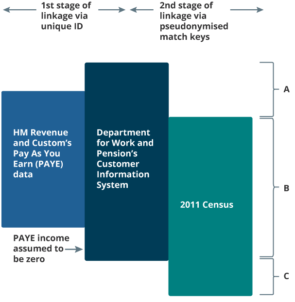
For the purposes of this research we have assumed a target census population of usual residents aged 16 to 64 years in private households. This target population is primarily driven by limitations in the data we currently have available, and subsequent research will consider alternative target populations, including in particular a wider age range. After matching, 7% of this target census population failed to link to the CIS (approximately 3 million individuals) and required imputation of income. This varied geographically, ranging from 4% to 23% at local authority level.
Within the census residuals (group C in Figure 1), we expect there to be people who had PAYE income greater than zero for the reference period and people who had PAYE income equal to zero. Where an individual had income greater than zero, they must have been a false-negative link, where the match between the CIS and census was missed. These individuals will also exist within the CIS residuals (group A in Figure 1), however, since group A will also contain individuals with positive income who were not usual residents as well as some individuals missed from the census, it is not possible to straightforwardly benchmark the census residuals against group A. Where an individual had PAYE income equal to zero, some will have been false-negative links (again appearing in the CIS residuals), but some will have also been genuine non-links. Genuine non-links will have occurred where individuals did not have a NI number and therefore did not appear in the CIS.
There are two types of individual who may have been usually resident on census day without a NI number. NI numbers are automatically allocated to all UK residents if a parent completes a Child Benefit form for them as a child. Individuals not automatically allocated a NI number need to apply for one if they intend to work, apply for a student loan or claim benefits. Therefore, the two types of individual without a NI number are:
migrants who moved to the UK and did not apply for a National Insurance number; this may have been because: they had no intention of ever working, claiming benefits or applying for a student loan; they had not completed the application process yet; or they had come to the UK to work from an European Economic Area (EEA) country but were getting paid by an organisation in that country, and were paying taxes there
UK residents whose parents did not complete a Child Benefit form for them and have had no reason to apply for a NI number yet, for example, they have never worked, claimed benefits or applied for a student loan
All these individuals should be imputed with zero PAYE income. While we do not have equivalent individuals without a NI number in our donor population (the census-CIS links), we can impute zero income values as we do have individuals within our linked population with a PAYE income of zero (for example, individuals not currently in the labour market), if we base the imputation upon auxiliary census variables that predict income. Information provided to us by DWP also indicates that we expect the number of individuals without a NI number to be small.
The Missing at Random assumption
An important assumption behind the validity of donor-based methods is that the data are Missing at Random (MAR), meaning the probability of missingness and missing values can be predicted from the observed data. Donor-based methods handle these situations well and MAR is therefore considered an "ignorable" missing data mechanism (Rubin, 1976).
To assess whether the linked administrative data supported this assumption, characteristics of the linked census-CIS data were compared with characteristics of the census residuals. This established whether certain characteristics explained missingness, but also whether certain characteristics, or combinations of characteristics, were observed within the census residuals that were not observed within the linked data, indicating the presence of subpopulations. Differences between the two datasets did indicate that some subpopulations were over-represented in the residual data (for example, students and migrants) indicating a non-response bias (or in this case, linkage bias) did occur (Figures 2 and 3).
Figure 2: Distribution of length of residence in the UK in the linked dataset and the residual dataset
Ages 16 to 64 years
Source: Office for National Statistics
Download this chart Figure 2: Distribution of length of residence in the UK in the linked dataset and the residual dataset
Image .csv .xls
Figure 3: Distribution of activity last week in the linked dataset and the residual dataset
Source: Office for National Statistics
Download this chart Figure 3: Distribution of activity last week in the linked dataset and the residual dataset
Image .csv .xlsCrucially, however, there was overlap in all characteristics, and the absolute size of all groups within the linked data was still larger than within the residuals. Differences in the characteristics of the linked data and the residuals may also explain why the linkage rate between the CIS and the census varied geographically, for example, areas with large proportions of migrants or students may have lower linkage rates.
To further assess the MAR assumption, relationships between the target and the observed census variables were also explored. Results indicated that the target variable was predictable from the observed census data, for example, individuals with higher-level qualifications were more likely to have higher incomes, as were individuals who were in good health. Combined with the previous results, these findings suggest that unbiased imputation should be possible if auxiliary information that explains distributional differences is included in the imputation model. Previously, we also outlined a requirement for individuals with zero income to be in our linked donor pool. It was therefore encouraging to see that there were many records in the donor pool with an income value of zero, and that these zeros were predictable from the observed census data.
Nôl i'r tabl cynnwys3. Imputation
Methodology
Census data contain many potential auxiliary variables, however, including all these variables in the imputation model was not feasible in the first stage of this work because of constraints on processing power and time, and the fact that including too many variables can lead to an insufficient number of donors in the imputation cells. Van Buuren and Groothuis-Oudshoorn (2011) recommend including three types of auxiliary variable:
variables that will be used for multivariate analysis (for example, correlations) after imputation
variables related to missingness of the target variable
variables that predict the target variable
Identifying variables that fulfil the first criterion is difficult, as it is hard to know how the imputed census data will be used after imputation. De Vaal (2016) discusses this challenge and describes how failing to include all relevant analysis variables in the imputation model can lead to incorrect conclusions being drawn, as multivariate relationships will not be retained. For this research, age and sex were identified as important analysis variables and were included as auxiliary information, however, future research should consider whether other variables should also be included for this reason.
Identifying variables to include under the second and third criteria was also a challenge, as early analysis revealed that many census variables were related to either missingness or values of the target variable. Although including all these variables would have strengthened the Missing at Random assumption and would have ensured all multivariate relationships were retained, as before, their inclusion in the model was not feasible because of restrictions on processing power. Instead, we explored the use of decision trees to select our auxiliary information, an approach that has previously been tested by both Statistics New Zealand (Zabala, 2015) and Statistics Canada (Stelmack, 2018). To do this, we used classification and regression tree (CART) analysis (Breiman, 1984) implemented in R using the Rpart package (Therneau and Atkinson, 2015).
Haziza and Beaumont (2007) explain that decision trees can be used in imputation to specify imputation classes because they allow data to be split into homogeneous groups with respect to a target variable (each "terminal node" of a tree represents an imputation class). In the context of hot deck imputation, donor pools are analogous to imputation classes, so decision tree algorithms can potentially be used directly to partition records and construct appropriate donor pools based on auxiliary variables present in both the donors and recipients (Andridge and Little, 2010).
With nearest-neighbour donor-based imputation, we cannot use decision trees to directly partition the donor pool, but we can use them to help identify appropriate auxiliary variables, or to pre-emptively identify imputation classes for our target variable, which can then be used to create a new categorical auxiliary variable that is included in the imputation model, with levels corresponding to the terminal nodes of the decision tree. Here, we tested the second approach, as it required fewer auxiliary variables to be included and was therefore quicker and required less processing power. A classification tree was used to predict missingness of the target variable and a regression tree was used to predict value.
This resulted in two new categorical variables to be included in the model. These are the census variables used in construction of the decision trees for one geographical area of England and Wales (Eastleigh, Southampton and Test Valley).
Classification tree predicting missingness
Country of birth
Second address indicator
Student accommodation
Regression tree predicting income value
Age
Economic activity
Hours worked
Industry
NS-SEC
Occupation
Transport to work
Three different imputation models were then run on this geographical subset of the 2011 England and Wales Census data using a version of nearest neighbour hot deck imputation coded in SAS. The models run were:
Baseline imputation model - imputing banded Pay As You Earn (PAYE) income amount using only age and sex as auxiliary information
Income band imputation - imputing banded PAYE income amount using age, sex and two categorical variables produced by the previously described decision trees as auxiliary information
Income value imputation - imputing continuous PAYE income amount using all variables described in 2 as auxiliary information as well as including the imputed income band from 2 as a must-match variable
Empirical evaluation
Firstly, an empirical evaluation was performed on the geographical subset of census data (Eastleigh, Southampton and Test Valley) where real missingness was imputed. After each run, all records were successfully imputed. The distribution of annual PAYE income amount for the imputed records was compared with the distribution of the observed records and the overall pre- and post-imputation distributions were also compared.
Differences in the distributions were not necessarily problematic, as under our Missing at Random assumption we expected differences to arise because of non-response bias. To interpret whether these differences were problematic, we must consider whether the differences were what we expected given what we know about the census residuals and the missing data process. In this situation, we expected a larger percentage of the imputed records to fall within the lower income bands compared with the observed data, as the characteristics of the census residuals (for example, students and migrants) were associated with having lower incomes.
Figure 4 shows that after imputing annual PAYE income band, a larger percentage of the imputed data fell within the two lowest income bands compared with the observed data. For example, in the observed data, 12% of individuals were in the £0.01 to £5,000 income band, whereas after income band imputation nearly 25% of the imputed data were in this band. This is then reflected in Figure 5, where we see that a larger percentage of individuals overall fell within the two lowest income bands after imputation. These changes were in line with our expectations given what we know about the residuals and the missing data process.
Changes in the distribution of continuous PAYE income amount were also compared before and after imputation. As expected, median PAYE income amount decreased following imputation, from £8,897 pre-imputation to £8,144 post-imputation.
Figure 4: The distribution of Pay As You Earn (PAYE) income band for the observed records and the imputed records
Ages 16 to 64 years, Eastleigh, Southampton and Test Valley
Source: Office for National Statistics
Download this chart Figure 4: The distribution of Pay As You Earn (PAYE) income band for the observed records and the imputed records
Image .csv .xls
Figure 5: The pre- and post-imputation distributions of Pay As You Earn (PAYE) income band
Ages 16 to 64 years, Eastleigh, Southampton and Test Valley
Source: Office for National Statistics
Download this chart Figure 5: The pre- and post-imputation distributions of Pay As You Earn (PAYE) income band
Image .csv .xlsChanges in the multivariate relationship between PAYE income amount and other census person variables were also examined. To do this, simple regression analyses were performed, and the regression coefficients were compared pre- and post-imputation (ordered probit regression was applied to the banded income amount and linear regression was applied to the continuous income amount, with dummy coding of nominal predictors). Any changes in the regression coefficients were assumed to indicate a change in the multivariate relationship.
After imputing banded PAYE income amount, differences in the pre- and post-imputation coefficients were small and the direction of all coefficients stayed the same, indicating that relationships were maintained. However, after imputing continuous PAYE income amount, the difference in some coefficients was quite large, indicating the imputation may have changed some multivariate relationships (see Coefficients from a generalised linear model predicting PAYE income amount from family status section). These findings suggest that auxiliary information included in the model was not sufficient when imputing continuous PAYE income amount, supporting De Vaal's (2016) argument that all variables that will be used for subsequent analysis should be included in the imputation model.
As well as assessing the distributional accuracy of the model, the donors and imputation variance introduced by the model were also reviewed. The median number of donors in each imputation class after the baseline imputation was 13,612, after income band imputation was 661 and after income value imputation was 95. Including the additional auxiliary information decreased the median number of donors available, however, in all instances the number of donors was reasonable, based on a rule of thumb that at least 30 potential donors should be available in each imputation class. The distance between the donors and the recipient records was also encouraging, with at least 95% of recipient groups matching the donors exactly, with the remaining groups only failing to match on one auxiliary variable.
The imputation variance that was introduced for each category of the target variable was also calculated assuming a multinomial distribution (Evans and others, 2000), taking into account the fact that donors were sampled without replacement. We wanted some imputation variance to be introduced, to reflect the uncertainty in the imputation, however, too high variance would indicate that the model had not sufficiently accounted for variance in the target variable or that it had not found appropriate donors. Results of this were also encouraging, with coefficients of variation ranging from 0.1% to 1.2% across the bands after income band imputation.
Overall, the empirical evaluation demonstrated that a nearest-neighbour donor-based imputation approach was able to successfully impute all records and maintain key conditional distributions, accounting for non-response bias. Including additional auxiliary information in the model improved the imputation based upon what we know about the census residuals and the missing data mechanism. However, changes to some multivariate relationships after imputation indicated that auxiliary information included in the model was not optimised when imputing a continuous PAYE income variable.
Simulation study
To further evaluate performance of the donor-based method, a simulation study was performed. The linked census-CIS data was used as a benchmark dataset and missingness was introduced according to the results of the classification tree that predicted missingness of the target variable. Allocating missingness in this way attempted to replicate the MAR mechanism observed in the full linked dataset, where the probability of missingness depended upon the observed census data. A prototype dataset was created with 7% of the target variable missing. This was then imputed according to the three imputation models, 10 times each.
Figure 6: Distribution of the true values for the missing records with the distribution of the imputed values following baseline imputation and income band imputation for simulation run 1
Ages 16 to 64 years, Eastleigh, Southampton, Test Valley
Source: Office for National Statistics
Download this chart Figure 6: Distribution of the true values for the missing records with the distribution of the imputed values following baseline imputation and income band imputation for simulation run 1
Image .csv .xlsFigure 6 shows that, in line with the conclusions of the empirical evaluation, the income band imputation was able to recover the true distribution of income bands well. As well as assessing distributional accuracy, the simulation study also enabled us to examine predictive accuracy of the model. Whilst only the maintenance of conditional distributions is required for the census, analysis of predictive accuracy provides further validation of the method.
Figures 7 and 8 show the distribution of differences between the true and imputed values following one run of both the baseline and income band imputations. Overall, the distributions were as expected, with a symmetrical peak around a difference of zero, demonstrating that the imputation was not biased. Encouragingly, the narrower distribution shown in Figure 8 also shows that including the extra auxiliary information improved the predictive accuracy of the model compared with the baseline. After the baseline imputation, the correct income band was imputed for 20% of records, rising to 29% after including the additional auxiliary information. Figure 9 shows the distribution of the differences between the true and imputed values following imputation of the continuous PAYE income variable. Again, the shape of the distribution is as expected with a symmetrical peak around zero.
Figure 7: Baseline imputation of income band
Source: Office for National Statistics
Download this chart Figure 7: Baseline imputation of income band
Image .csv .xls
Figure 8: Income band imputation
Source: Office for National Statistics
Download this chart Figure 8: Income band imputation
Image .csv .xls
Figure 9: Continuous income value imputation
Source: Office for National Statistics
Download this chart Figure 9: Continuous income value imputation
Image .csv .xlsThe distribution of differences for the remaining nine prototypes after each imputation were very similar. However, Table 1 shows there were differences in the income band or income value that was imputed for each missing record across the 10 iterations. This demonstrates that imputation variance was introduced at the record level.
After the baseline imputation, the average range of imputed PAYE income band for each record was 5.6, reducing to 4.2 after including the additional auxiliary information. After imputing continuous PAYE income amount, the average range was £6,553. The mean difference across the 10 iterations compared with the true value was also calculated for each record and averaged for the whole dataset. This also decreased after including the additional auxiliary information.
| Baseline imputation | Income band imputation | Income value imputation | |
|---|---|---|---|
| Mean range of imputed values | 5.6 bands | 4.2 bands | £6,553 |
| Mean absolute difference | 2.3 bands | 1.6 bands | £10,837 |
Download this table Table 1: The mean range and the mean absolute difference in imputed values averaged for the whole dataset, after imputing banded Pay As You Earn (PAYE) income and continuous PAYE income amount
.xls .csvThese findings suggest that a large amount of imputation variance was introduced at the record level, although variance did decrease after including additional auxiliary information. When considered alongside the fact that the true PAYE income band was only recovered for 29% of records, this suggests that predictive accuracy of the model was fairly low. This supports findings from the empirical evaluation, indicating that the auxiliary information included in the model was not sufficient to obtain high predictive accuracy despite achieving good distributional accuracy.
Nôl i'r tabl cynnwys4. Conclusions and recommendations
Here we have demonstrated that a nearest-neighbour donor-based imputation approach was able to successfully impute a linked person level dataset where the only source of missingness was linkage error. An administrative-based income variable linked to 2011 Census data was successfully imputed, and results of both an empirical evaluation and a simulation study show that including observed census data as auxiliary information in the model accounted for non-response bias and maintained conditional distributions.
However, findings also suggest that predictive accuracy of the model was quite low, and that not all multivariate relationships were maintained following imputation. This suggests that the decision-tree method used to create auxiliary variables was not sufficient to maintain all multivariate relationships. This means that, while it is possible to impute a linked income variable using the approach outlined in this article, it would not be reasonable to treat income in the same way as the collected census data and, for example, cross-tabulate it against all other census variables. To meet these additional aims, it may be necessary to include all variables identified by the decision tree, or required for subsequent analysis, in the imputation model.
Future research should therefore focus on whether including additional auxiliary information in the model improves predictive accuracy and the maintenance of multivariate relationships. To do this, imputation will be run using the Canadian Census Edit and Imputation System (CANCEIS) (Bankier and others, 1999) as this is able to handle many auxiliary variables well. This will be our priority area of research once the required data are available.
We will also consider the use of regression analysis to assess whether multivariate relationships are maintained, and regression analysis could also be used to select auxiliary variables, by identifying the strongest predictors of linkage error and income value. Other potential research areas are extending the simulation study presented here to evaluate the sensitivity of the model to different missing data mechanisms, for example, by introducing a Not Missing at Random data mechanism, where the missingness introduced depends on the income value itself. Finally, results of this donor-based approach should be compared with other machine learning and model-based methods, for example, regression imputation.
Nôl i'r tabl cynnwys5. Coefficients from a generalised linear model predicting PAYE income amount from family status
| Central London | Eastleigh, Southampton, Test Valley | |||||
|---|---|---|---|---|---|---|
| Pre- imputation | Post- imputation | Absolute difference (%) | Pre- imputation | Post- imputation | Absolute difference (%) | |
| Intercept | 25,748.70 | 24,278.58 | 1470 (6) | 13,516.06 | 11,818.00 | 1698 (13) |
| In a couple family: Member of couple | 14,637.35 | 14,504.62 | 133 (1) | 4,286.57 | 5,909.24 | 1623 (38) |
| In a couple family: Dependent child of one or both members of the couple | -25,680.80 | -24,177.90 | 1503 (6) | -13,249.80 | -11,532.30 | 1718 (13) |
| In a couple family: Non-dependent child of one or both members of the couple | -18,233.10 | -16,180.80 | 2052 (11) | -5,756.07 | -3,958.93 | 1797 (31) |
| In a lone parent family: Parent | -16,244.00 | -13,940.20 | 2304 (14) | -4,158.87 | -2,396.34 | 1763 (42) |
| In a lone parent family: Dependent child of parent | -25,665.30 | -24,175.20 | 1490 (6) | -13,297.90 | -11,582.20 | 1716 (13) |
| In a lone parent family: Non-dependent child of parent | -17,840.40 | -15,762.30 | 2078 (12) | -6,144.48 | -4,371.61 | 1773 (29) |
Download this table Table 2: Coefficients from a generalised linear model predicting PAYE income amount from family status
.xls .csv6. References
Abbott, O., Ralphs, M., and Jones, P. (2016). Large-scale Linkage for Total Populations in Official Statistics. In K. Harron, H. Goldstein, and C. Dibben (Eds.), Methodological Developments in Data Linkage, Wiley, pages 170 to 199
Aldrich, S., Wardman, L., and Rogers, S. (2012), The practical implementation of the 2011 UK Census imputation methodology (PDF, 361KB), Conference of European Statisticians, Work Session on Statistical Data Editing, United Nations Economic Commission for Europe, viewed 21 September 2020
Bankier, M., Lachance, M., and Poirier, P. (1999). A Generic implementation of the nearest neighbour imputation method. Proceedings of the Survey Research Methods Section. American Statistical Association, pages 548 to 553
Breiman, L. (1984). Classification and Regression Trees. New York: Routledge, viewed 21 September 2020
Evans, M., Hastings, N., and Peacock, B. (2000). Statistical Distributions (3rd edition). New York: Wiley, pages 134 to 136
Haziza, D., and Beaumont, J., F. (2007), "On the construction of imputation classes in surveys", International Statistical Review, Volume 75, pages 25 to 43
Office for National Statistics (2014), 2011 Census item edit and imputation process (PDF, 203KB), viewed 21 September 2020
Office for National Statistics (2020), Statistical design for Census 2021, England and Wales, viewed 1 October 2020
Rubin, D.B. (1976), "Inference and missing data", Biometrika, Volume 63, Number 3, pages 581 to 592
Statistics Canada (2017), Income Reference Guide, Census of Population, 2016, viewed 20 January 2020
Stelmack, A. (2018), On the Development of a Generalized Framework to Evaluate and Improve Imputation Strategies at Statistics Canada (PDF, 789KB), Conference of European Statisticians, Workshop on Statistical Data Editing, United Nations Economic Commission for Europe, viewed 21 September 2020
Therneau, T. and Atkinson, B. (2015), An introduction to recursive partitioning using the RPART routines (PDF, 401KB), Mayo Foundation, viewed 21 September 2020
Van Buuren, S., Groothuis-Oudshoorn, K. (2011), mice: Multivariate Imputation by Chained Equations in R, Journal of Statistical Software, Volume 45, Number 3, pages 1 to 67, viewed 21 September 2020
Zabala, F. (2015), Let the data speak: Machine learning methods for data editing and imputation (PDF, 734KB), Conference of European Statisticians, Work Session on Statistical Data Editing, United Nations Economic Commission for Europe, viewed 21 September 2020
Nôl i'r tabl cynnwys7. Collaboration
This research was produced in collaboration between the Methdology Division (Anna Summerbell, Andrew Taylor and Fern Leather) and the Statistical Design and Research Division (Matthew Greenaway).
Email: Admin.Based.Characteristics@ons.gov.uk
Nôl i'r tabl cynnwys