Cynnwys
- Authors
- Introduction
- Living Costs and Food (LCF) survey data and Classification of Individual Consumption by Purpose (COICOP) classification
- Classification of Individual Consumption by Purpose (COICOP) level assessment
- Small area estimation methods
- Small area estimation results
- Summary and recommendations
- Appendix
2. Introduction
Consumer price indices are used as a national measure of inflation, of which the Office for National Statistics' (ONS's) preferred and most comprehensive measure is the Consumer Prices index, including owner occupiers’ housing costs (CPIH). There has been interest in regional indices over many years and this led to an initial assessment of the feasibility of producing regional CPIH indices for comparison of inflation rates between regions (temporal indices), in contrast to spatial indices such as the Relative regional consumer price levels, which are used to compare the levels of prices between regions.
A major challenge in developing a regional CPIH is to estimate stable expenditure weights at the regional level. Weights are needed to combine information for different products, and the Classification of Individual Consumption by Purpose (COICOP) scheme is used as its basis. Expenditure weights for the national CPIH are derived from the National Accounts household expenditure data, which are derived from Living Costs and Food (LCF) survey data, market research data and other sources including administrative data. For regional expenditure weights, up until recently the only accessible source which can be used at the regional level is the LCF survey, which is the data source we focus on in this report. The recently published regional household final consumption expenditure is a data source that could also be integrated into developing a regional CPIH, which we leave for further research.
It has previously been shown that using direct estimates (that is, estimates based only on information about the region and period in question) of expenditure weights from the LCF result in a regional CPIH with unrealistically volatile year-to-year trends. This is at least partly due to small household sample sizes in the LCF at the regional level that cause a lack of stability in the estimates over time. It was concluded that the regional CPIH could not be constructed in the same way as the national CPIH, and that advanced methods would be required. One recommendation was that small area estimation (SAE) could be used to improve the temporal stability of the weight estimates. SAE methods would act to improve regional estimates by “borrowing strength” from other regions in a model-based framework. The aim of this report is to explore the potential suitability and benefits of using SAE for regional expenditure weights in a regional CPIH. In particular, the report focuses on:
which COICOP level is most appropriate for SAE to be performed
which COICOP categories benefit the most from SAE
how much temporal volatility of the regional CPIH can be reduced using SAE compared to established methods using direct estimation
identifying sources of volatility in the regional CPIH, which SAE cannot reduce
recommendations for further research into the development of a regional CPIH
While the focus of this report is on the expenditure weights, we acknowledge the importance of assessing the stability of the price estimates as well. A regional CPIH would require stable estimates for both the prices and the expenditure weights. Although it was suggested by Dawber and Smith (2017) that the expenditure weights contributed more volatility to the regional CPIH compared with the price quotes, this is yet to be fully investigated, which we leave for future research.
All measures of regional CPIH calculated in this report are experimental statistics, provided as part of the development process for the purposes of gathering feedback and for quality assurance. They are not fully developed statistics and are subject to changes. Therefore, caution should be used when interpreting the indices and they should not be used as the basis for decision-making in their current form.
Nôl i'r tabl cynnwys3. Living Costs and Food (LCF) survey data and Classification of Individual Consumption by Purpose (COICOP) classification
Living Costs and Food (LCF) survey data was obtained for the years 2006 to 2014. This included the household and individual level data files. The LCF data provide expenditure on products purchased by each sampled household in each of the 12 regions. These products are classified at the Classification of Individual Consumption by Purpose (COICOP)-plus level which are sub-categories of the COICOP 5 level according to European Classification of Individual Consumption according to Purpose (ECOICOP). An example of the COICOP classification is shown in Table 1, which also shows the terminology or labels for the different levels. The item level is also included, which is the lowest level of classification and sits below the COICOP hierarchy. Items are chosen by Office for National Statistics (ONS) to be representative within a COICOP 5 category. The COICOP-plus level is used in the LCF data to provide more detailed recording of expenditure items.
| Level | COICOP2 | COICOP3 | COICOP4 | COICOP5 | COICOP-plus | Item |
|---|---|---|---|---|---|---|
| Label | Division | Group | Class | Expenditure code | Category | - |
| Example | Food and non-alcoholic beverages | Food | Bread and cereals | Bread | Buns, crispbread and biscuits | White sliced loaf branded 750G |
| Code | 1 | 1.1 | 1.1.1 | 1.1.1.2 | 1.1.1.2.2 | - |
| Number | 12 | 47 | 117* | 307 | 367 | 731 |
Download this table Table 1: Example COICOP classification
.xls .csvThe aim is to estimate the mean (or equivalently the total) household expenditure in each of the 12 regions of the UK (which is used to weight the prices at the same level). These estimates can be adjusted for consistency with a range of other data sources in a balancing process, and then converted into relative weights (measured in parts per thousand (ppt) of expenditure). ONS makes these adjustments to account for underreporting in the LCF survey, for example, for alcohol and tobacco, as well as to incorporate other data sources. We refer to these weights as the adjusted weights, as opposed to unadjusted weights which would be derived solely from the LCF data. The adjusted weights are combined with the regional price quotes to give a regional Consumer Prices Index, including owner occupiers’ housing costs (CPIH).
It should be noted that because this report focuses on estimating expenditure weights from LCF data only, not all COICOP classes will be represented. Five classes in total are not reported in the LCF survey. This is why other non-LCF data sources are also used in construction of CPIH. Most importantly, COICOP Class 4.2 “Owner occupiers housing costs” is not represented. Since the CPIH is comprised of all the same classes as the Consumer Prices Index (CPI) with the addition of Class 4.2, the index generated in this report is closer to the CPI rather than the CPIH. We leave the investigation of small area estimation (SAE) applied to Class 4.2 weight estimation for further research.
Note that the LCF data for 2006 was deficient in many COICOP classes and hence was removed completely for all further analyses. This left eight years data from 2007 to 2014.
Nôl i'r tabl cynnwys4. Classification of Individual Consumption by Purpose (COICOP) level assessment
Before applying small area estimation (SAE) methods, the level of estimation must first be chosen. We focus on determining whether the Classification of Individual Consumption by Purpose (COICOP)-plus level or COICOP 4 level is better for SAE. This reflects the lowest and highest levels which are practical for use (COICOP 5 could also be used if a middle ground appears to be optimal). The choice of level depends on two primary aspects: sample sizes and the regional basket size based on expenditure. SAE should only be applied if there is a large enough sample size from which model-based estimates can be useful as well as having a non-trivial amount of expenditure, for example, over 0.5 parts per thousand (ppt).
When we consider the sample size we must consider two levels; the household level and the COICOP level. The main sampling unit is the household, from which the expenditure is recorded, and later classified according to COICOP. The sample size of households at the region level is small enough to be of concern, with the Living Costs and Food (LCF) sample sizes shown in Table 2 for 2007 to 2014. On average the North East and Wales have the smallest number of households sampled, compared with the South East which has approximately three times the number. Northern Ireland has had a very small sample size since 2010, but this was boosted from the 2016 to 2017 survey year. It is also worth noting the decreasing trends over time for all regions.
| LCF year | North East | North West | Yorkshire and Humberside | East Midlands | West Midlands | East | London | South East | South West | Wales | Scotland | Northern Ireland |
|---|---|---|---|---|---|---|---|---|---|---|---|---|
| 2007 | 257 | 603 | 525 | 458 | 500 | 551 | 528 | 839 | 499 | 279 | 501 | 596 |
| 2008 | 235 | 592 | 491 | 405 | 469 | 532 | 472 | 806 | 502 | 265 | 500 | 574 |
| 2009 | 236 | 582 | 484 | 393 | 527 | 499 | 464 | 701 | 518 | 272 | 544 | 602 |
| 2010 | 258 | 596 | 485 | 413 | 470 | 515 | 476 | 679 | 495 | 261 | 468 | 147 |
| 2011 | 283 | 647 | 521 | 455 | 526 | 543 | 536 | 761 | 507 | 251 | 500 | 161 |
| 2012 | 262 | 623 | 521 | 425 | 513 | 563 | 490 | 783 | 493 | 266 | 483 | 171 |
| 2013 | 251 | 585 | 462 | 424 | 526 | 497 | 480 | 681 | 429 | 246 | 412 | 151 |
| 2014 | 255 | 588 | 459 | 440 | 470 | 498 | 407 | 740 | 468 | 222 | 434 | 152 |
| Mean | 254.6 | 602 | 493.5 | 426.6 | 500.1 | 524.8 | 481.6 | 748.8 | 488.9 | 257.8 | 480.3 | 319.3 |
Download this table Table 2: Sample size of households for Living Costs and Food (LCF) data, 2007 to 2014
.xls .csvAt each household the expenditure is reported in detail and coded at the COICOP-plus level, so this is the lowest level available. This means that if all sampled households purchase from a given COICOP-plus category, then the number of expenditure observations will match the household sample size. However, there are always some households that do not purchase products from some of these COICOP-plus categories, so the number of non-zero observations at the COICOP-plus level will always be less than the number of observed households. If a large majority of households do not make purchases from a given COICOP-plus category then this will be problematic since only a few sampled households will have to represent the entire region. It may be better to instead use a higher COICOP level such as the class level, where the purchases are aggregated, providing more non-zero expenditure observations to use for estimation.
For the remainder of the report we use the term “observation” to specifically mean any non-zero expenditure recorded from a given COICOP category or class. Observations of zero expenditure are still used for estimates, but for simplicity we do not refer to these as observations. For example, if 250 out of 300 households in a region had recorded expenditure for a given COICOP-plus category then we would say there were 250 observations. Similarly, we may say there were 1000 observations out of 300 households for a given region and COICOP class. This is because, for the higher COICOP level of class, there can be multiple observations within a household.
Multiple observations within a COICOP class occur because a COICOP class contains a number of COICOP-plus categories within it. This means the COICOP-plus categories can be aggregated at the COICOP class level, leading to more non-zero regional expenditures. Some classes have more COICOP-plus categories than others. For example, the COICOP Class 1.1.1 “Bread and cereal” includes seven COICOP-plus categories including rice, bread, buns and biscuits, cereal and pasta. This COICOP class is well represented in the LCF data since these are all commonly consumed products. Comparatively, the COICOP Class 7.3.3 “Passenger transport by air” is purchased relatively rarely, and furthermore it is separated into only two COICOP-plus categories, domestic and international air travel. So it is both the frequency and broadness of classes like 1.1.1 which provide relatively large numbers of observations. The number of observations for each of the 87 COICOP classes based on the 2014 LCF data are shown in Table 4 in the Appendix. Note that some of these classes such as 4.2 “Owner occupiers’ housing costs” are not expected to be recorded in the LCF survey so are expected to be zero.
To compare the two COICOP levels and the corresponding observation number, we focus on the North East region, which has the smallest mean sample size as shown in Table 2. Figure 1 and Figure 2 show the North East mean number of observations over the eight years of LCF data for the COICOP-plus level and the COICOP class level respectively. To compare the two, a reference line at 30 observations is included in both figures (typically 30 is arbitrarily considered to be the boundary between having a “small” or “not-small” sample size). On both levels, there are a number of categories with fewer than 30, but more so for the lower level COICOP-plus. For this reason, more stable estimates are likely to come from the COICOP class level. We also observe that generally, Divisions 01 (Food and non-alcoholic beverages) and 02 (Alcoholic beverages and tobacco) are relatively well represented, whereas Divisions 04 (Housing, water, electricity, gas and other fuels) and 10 (Education) are particularly poorly represented – at least partly because of the two-week diary approach to data collection in the LCF.
Figure 1: Mean number of observations from 2007 to 2014 for each COICOP-plus group, North East region
Source: Office for National Statistics
Download this chart Figure 1: Mean number of observations from 2007 to 2014 for each COICOP-plus group, North East region
Image .csv .xls
Figure 2: Mean number of observations from 2007 to 2014 for each COICOP class, North East region
Source: Office for National Statistics
Download this chart Figure 2: Mean number of observations from 2007 to 2014 for each COICOP class, North East region
Image .csv .xlsAt the COICOP class level, we can see in Figure 2 that Division 01 “Food and non-alcoholic beverages” is well represented, as well as Classes 5.6.1 “Non-durable household goods”, 11.1.1 “Restaurants and cafes” and 12.1.2 “Appliances and products for personal care”. On the other hand, a total of 5 out of 87 classes (5.7%) have no representation in the LCF data for the presented years.
In 2014, 19 out of 87 classes (21.8%) had at least one region with no observations. For COICOP-plus, it was 32.2% in 2014. If we argue that when there are fewer than 10 observations estimates are likely to be too unreliable, that would mean 35 out of 87 classes (40.2%) will not have reliable estimates for at least one region in 2014. For COICOP-plus, this was 60.2%. Similarly, 51 out of 87 classes (58.6%) have fewer than 30 observations for at least one region in 2014. For COICOP-plus, this was 76.6%. Clearly, there is a large amount of variability between the number of observations across the different COICOP classes and categories. Some classes from Division 01 have enough observations to provide quite reliable direct estimates for the regional level, however many classes do suffer from a lack of observations.
Although the number of observations is an important consideration, the actual expenditure must also be considered. The problem of few observations will be compounded when there is higher expenditure. For example, in the North East, COICOP Classes 6.2.2 “Dental services” and 12.4 “Social protection” both receive fewer than 10 observations on average each year, but the former comprises of 3.0ppt of the total unadjusted expenditure compared with 9.8ppt for the latter. Since these estimates are to ultimately provide weightings for the price quotes, the higher weights will have greater impact on the resulting regional index. For this reason, estimates for Class 12.4 have greater potential to cause instability to the regional index compared with Class 6.2.2. Hence we consider the expenditure estimates as well as the sample sizes for each COICOP category.
The North East mean expenditure in parts per thousand for the COICOP-plus and COICOP class level are shown in Figure 3 and Figure 4 respectively, with a reference line added at 10ppt (1%) for comparison. It should be noted that the other regions do not have substantially different expenditure distributions and hence share somewhat similar trends to the North East. We compare the expenditure of the two COICOP types for two reasons. Firstly, we assume that the higher the relative expenditure, the more reflective it will be of the regional economy, making it more plausible to predict using economic variables. Secondly, the fewer regions with non-zero expenditure the better the SAE model, since zeroes can violate model assumptions.
Figure 3: Unadjusted estimates of relative expenditure by COICOP-plus group, North East region
Office for National Statistics
Source: Office for National Statistics
Download this chart Figure 3: Unadjusted estimates of relative expenditure by COICOP-plus group, North East region
Image .csv .xls
Figure 4: Unadjusted estimates of relative expenditure by COICOP class, North East region
Source: Office for National Statistics
Download this chart Figure 4: Unadjusted estimates of relative expenditure by COICOP class, North East region
Image .csv .xlsWe can see that the parts per thousand (ppt) for the COICOP-plus categories are all mostly far below the 1% reference line. COICOP classes also have a high proportion of relatively small expenditure, but it is much less. The North East median COICOP-plus category has 0.9ppt compared to 5.9ppt for the median COICOP class. Furthermore, Figures 5a and 5b compares the proportion of categories that are above 0.5 ppt (0.05%) for COICOP-plus and COICOP classes. While the COICOP-plus maintains only around 60% across 2007 to 2014, the COICOP classes maintain around 80%. This substantially larger relative expenditure for COICOP classes is a further indication that the class level will be more suitable for modelling.
Figure 5a: Proportion of COICOP classes which have parts per thousand threshold above 0.5 (0.05%), UK regions

Source: Office for National Statistics
Download this image Figure 5a: Proportion of COICOP classes which have parts per thousand threshold above 0.5 (0.05%), UK regions
.png (22.5 kB) .xls (27.6 kB)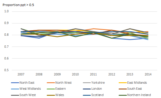
Figure 5b: Proportion of COICOP-plus categories which have parts per thousand threshold above 0.5 (0.05%)
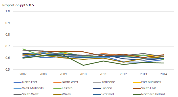
Source: Office for National Statistics
Download this image Figure 5b: Proportion of COICOP-plus categories which have parts per thousand threshold above 0.5 (0.05%)
.png (22.2 kB) .xls (38.9 kB)
Based on the assessment of the number of observations and the relative expenditure we argue that modelling should occur at the COICOP class level, instead of the COICOP-plus level. We do this for the following reasons:
the COICOP class level results in fewer non-zero regional expenditure estimates
similarly, the COICOP class level results in higher mean regional expenditure making it better for SAE models
If SAE is to improve the estimation of expenditure weights it will be more likely to do so at a higher level of aggregation.
Nôl i'r tabl cynnwys5. Small area estimation methods
Having identified that estimating aggregated expenditure at the Classification of Individual Consumption by Purpose (COICOP) class level is likely to be the most suitable approach for small area estimation (SAE), we now describe the modelling methods. The aim of the SAE models is to provide improved stability of expenditure over time, making the expenditure estimates better weights for the regional Consumer Prices Index, including owner occupiers’ housing costs (CPIH).
Fay-Herriot models
The SAE method used for expenditure estimation was the Fay-Herriot (FH) model, which is described in this section.
Let yij denote the total household expenditure in pounds for household j in region i for each COICOP class and each year. Suppose that ni is the household sample size for region i, and so the direct estimate of the mean household expenditure θi can be estimated using:
For households that do not purchase items within the COICOP class, then yij=0. For many households across many COICOP classes there is zero expenditure. The consequence of this is that modelling at the household level becomes problematic, as large proportions of zeros lead to violations of typical distributional assumptions. For example, the distribution of expenditure for households that did spend something may be approximately normally distributed, however the addition of the considerable proportion of zeroes from households who did not spend anything leads to a zero-inflated distribution. A common way of avoiding this complexity is to model at an aggregate level, which in this case would be the region level. This would ensure there is not a large number of zeroes, except rare occurrences where all households within a whole region have no expenditure for a COICOP class. A commonly used region-level model for SAE is a FH model. The FH model is based on two stages. The first stage simply models the sampling variation, hence:
where the sampling errors εi are assumed to be independent and normally distributed. We can estimate the variance parameter using bootstrapping. If there are no observations for at least some regions then the assumption of normality will be less likely to justify.
The second stage of the FH model is to fit a linear model which can be used to predict θi:
where xiT denotes the region-level covariates, β denotes the regression parameter vector, and ui represents the random effects which, similarly to εi, are assumed to be independent and normally distributed. The combination of the two stages of modelling leads to the combined FH model:
The estimates of these unknown parameters can be estimated using a standard linear random-effects model. From this the FH estimates can be derived as:
Estimates of the precision of the FH estimates can be made using the mean squared error (MSE) which is estimated using restricted maximum likelihood (REML).
The total household expenditure for a region can easily be found by multiplying the mean household estimate by the total number of households in the region, which is estimated by Office for National Statistics (ONS).
One of the strengths of SAE is borrowing strength from other areas. This is done by using the association between the region-level covariates and the regional expenditure. Region-level associations strengthen each individual region by using the region-level covariates, which are assumed to be quite informative. A limitation faced with only having twelve regions is that these associations are determined with only twelve observations. With such a small number an association can occur by chance quite easily.
Variable selection
The Living Costs and Food (LCF) survey provides a large number of variables at the region level which can be used to estimate expenditure. These variables relate to wealth, household compositions and types, and income. For a FH model to be effective at estimating expenditure, the region-level covariates should be predictive of the expenditure of the COICOP classes. The challenge is to select the best combination of variables which ensures the relationship is predictive but not over-fitted to the sampled data. This over-fitting is especially a concern since there are only twelve regions, hence twelve points from which to fit a model. Furthermore, the covariates should not have high multicollinearity, as this can greatly exaggerate over-fitting. Over-fitting will lead to small area estimates with under-estimated precision, as well as overly biased point estimates, so the explanatory variables must be selected carefully.
The variables were chosen by first pooling all years of LCF data. The idea is to select variables that predict expenditure well for all years and that those variables be used in the model every year. This will ensure consistency across time. A forward selection approach was used to select the variables for each COICOP class. First the most predictive variable is added to the null model and then a second variable is selected if it significantly improves the model. This is repeated until at most five variables are selected. We made five the maximum since any more seemed superfluous when estimating twelve regions. At each step the multicollinearity was assessed using the variance inflation factor (VIF). If the VIF was greater than ten then no more variables were added. This ensured that a minimal number of variables were selected and that none of the variables were highly collinear.
Model assessment
A FH model relies on a strong level of prediction with explanatory variables. The coefficient of determination, or R2, is a commonly used statistic that measures the predictive ability of a model. More formally, R2 measures the percent of variation explained by the predictor variables. The closer it is to one, the better the FH model will be. Figure 6 shows the mean R2 values of the fitted models for each COICOP class. It shows that in Divisions 01 and 02 the R2 is generally high, but there are high and low values for other Divisions. As a rule of thumb, an R2 less than 0.2 is unlikely to provide substantial improvements over the direct estimator, so for example COICOP Class 12.6.2 “Other financial services” with a mean R2 of 0.03 will not likely be substantially improved using SAE.
Figure 7 shows the relationship between the mean R2 and the parts per thousand of the COICOP class. As previously assumed, the more expenditure that is recorded, the better the model predictions. This is because the expenditure is more likely to reflect economic conditions in that region. For example, restaurant and café purchases would be expected to be high when economic conditions are good, whereas rarely purchased kitchen appliances would not be expected to be as closely associated with economic conditions.
Figure 6: Mean R2 over 2007 to 2014 for each COICOP class
Source: Office for National Statistics
Download this chart Figure 6: Mean R^2^ over 2007 to 2014 for each COICOP class
Image .csv .xls
Figure 7: Mean expenditure parts per thousand over regions and years against the mean R2 of the regression model for each COICOP class
Source: Office for National Statistics
Download this chart Figure 7: Mean expenditure parts per thousand over regions and years against the mean R^2^ of the regression model for each COICOP class
Image .csv .xlsWith the FH models fitted, it remains to be seen what the effect on the stability of the expenditure estimates is when we use the model predictions in place of the direct estimates.
Nôl i'r tabl cynnwys6. Small area estimation results
We assess the effects of small area estimation (SAE) in two ways. First we compare the Fay-Herriot (FH) and direct estimates and then we assess the adjusted weights that are derived from these estimates. We make this assessment through observing the effects the adjusted weights have on the regional Consumer Prices Index (CPI).
To assess the the effect that FH estimation has on the expenditure we first measure how different they are from the direct estimates. Figure 8 focusses on the North East region, showing the percent difference between the FH and direct estimate, averaged over the eight years. This reveals up to a 30% difference in the estimates with many Classification of Individual Consumption by Purpose (COICOP) classes showing non-trivial relative differences. Clearly FH estimation has some effect, but it is unclear what effect this is. Before investigating this, we first need to explain the spaces in Figure 8 where no percent difference is shown. This occurs for COICOP classes where FH estimates could not be calculated due to too many regions with no observations. Even if only a few regions have zero expenditure it may cause the FH model to not converge resulting in no FH estimates for all regions. In total, FH estimates could not be calculated for 16 of the 87 COICOP classes (18.4%). These classes are highlighted on the first column in Table 5 in the Appendix and are removed for the remaining results.
Figure 8: Mean percent difference between Fay-Herriot estimate and direct estimate, North East region
Source: Office for National Statistics
Download this chart Figure 8: Mean percent difference between Fay-Herriot estimate and direct estimate, North East region
Image .csv .xlsThe primary purpose of utilising FH estimation on expenditure is to improve the stability of the estimates over time. We expect that expenditure patterns are in reality rather stable, and change slowly as consumer spending is influenced by changes in products and their availability, particularly at higher levels of aggregation in COICOP. Therefore we judge that the more stable the estimates are over 2007 to 2014, the better the estimates are and the more stable the regional Consumer Prices Index, including owner occupiers’ housing costs (CPIH) will be. Note that some expenditure patterns may actually vary substantially over time, so expert opinion on what level of variability is realistic would need to be considered too. To measure this stability over time we measure the variability of the yearly estimates of expenditure; this will include a small element of real change in expenditure patterns, but we expect that this is much smaller than the random variation we are trying to smoothen using SAE. Typically the standard deviation or variance is used to measure variability, however this will not be appropriate in this case. This is because the variance is greater for COICOP classes with higher expenditure. To accommodate this, we use the coefficient of variation (CV) which is the standard deviation divided by the mean. This ensures the measure is standardised by the amount of expenditure, hence making the metric comparable across all COICOP classes.
So we use this “temporal” CV to compare the stability of the FH estimates with the direct estimates. The lower the temporal CV, the more stable the estimates over time. Figure 9.1 and 9.2 compare this temporal CV for the North East region, with Figure 9.1 showing the CVs for the direct and FH estimates and Figure 9.2 showing the actual difference between them. These actual differences in the temporal CVs between direct and FH estimates are then shown for all regions in Figure 10. A zero difference indicates no improvement in temporal stability due to FH estimation, whereas positive differences show an improvement. Although infrequent, a negative difference suggests FH estimates are less stable, which may occur for COICOP classes with ill-fitted models.
Figure 9.1: Difference in temporal coefficient of variation between direct and Fay-Herriot estimates (second plot shows differences between the two bars in the first plot), North East region
Source: Office for National Statistics
Download this chart Figure 9.1: Difference in temporal coefficient of variation between direct and Fay-Herriot estimates (second plot shows differences between the two bars in the first plot), North East region
Image .csv .xls
Figure 9.2: The differences between the two bars in Figure 9.1
Source: Office for National Statistics
Download this chart Figure 9.2: The differences between the two bars in Figure 9.1
Image .csv .xlsThe differences in the temporal CV between FH and direct estimates is almost always positive for every COICOP class and region, indicating an improvement in stability due to FH estimation. The biggest exception is with the North East for COICOP Class 9.1.2 “Photographic, cinematographic and optical equipment” which was only recorded in the Living Costs and Food (LCF) survey very rarely (ranging between one and six) each year. There is clearly a very small difference for Divisions 01 and 02 in all regions, highlighting how SAE has a smaller effect for classes which already have many observations from the LCF. The region with the most observations, the South East, also shows the smallest differences, as would be expected. Figure 10 does not reveal any clear patterns on which COICOP classes are consistently showing large improvements due to FH estimation. To identify these classes the mean CV differences were taken across the regions and the top ten highest differences reported in Table 3, along with other attributes of those classes.
Figure 10: Difference in temporal coefficient of variation between direct and Fay-Herriot estimates, all UK regions
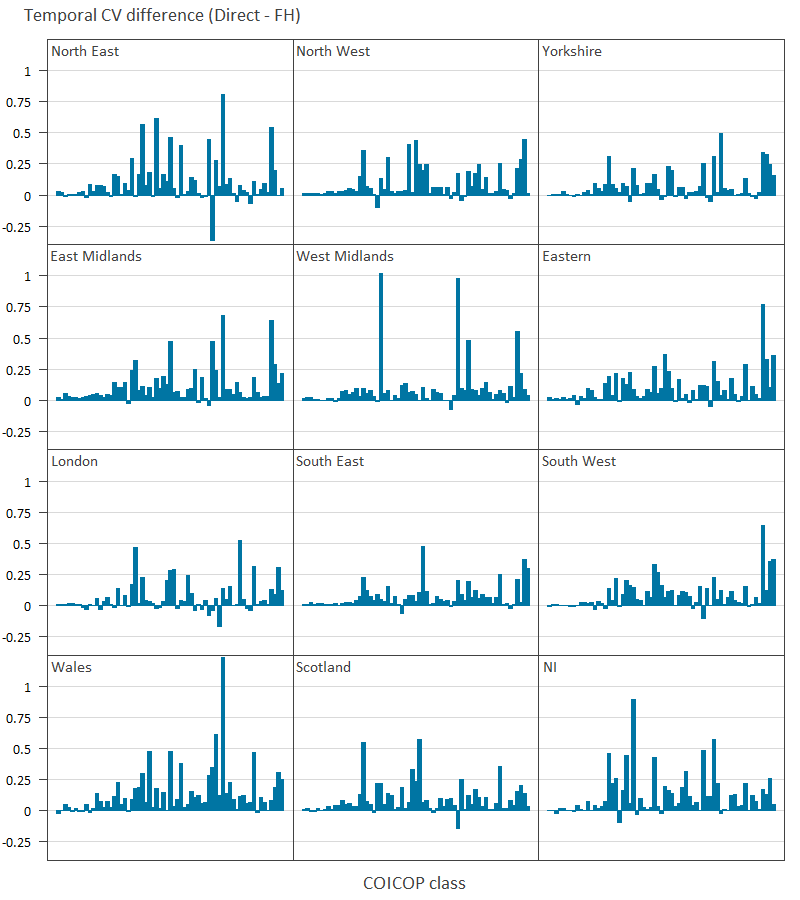
Source: Office for National Statistics
Download this image Figure 10: Difference in temporal coefficient of variation between direct and Fay-Herriot estimates, all UK regions
.png (15.6 kB) .csv (10.2 kB)
| COICOP class | Temporal CV difference | Mean number of observations | Mean ppt | Mean R² |
|---|---|---|---|---|
| 9.2.1 | 0.44 | 6.8 | 2.97 | 0.22 |
| 12.3.1 | 0.37 | 60.3 | 6.55 | 0.22 |
| 5.3.1/2 | 0.27 | 40.8 | 11.46 | 0.14 |
| 5.1.1 | 0.27 | 63.1 | 3.98 | 0.38 |
| 3.1.4 | 0.25 | 15.8 | 1.05 | 0.52 |
| 10 | 0.23 | 11.5 | 1.32 | 0.4 |
| 12.5.2 | 0.23 | 9.8 | 0.39 | 0.33 |
| 6.2.2 | 0.22 | 20.7 | 5.08 | 0.65 |
| 12.4 | 0.2 | 23.5 | 12.09 | 0.47 |
| 9.1.2 | 0.2 | 7.4 | 1.95 | 0.14 |
Download this table Table 3: Top ten COICOP classes with most improvement in stability due to Fay-Herriot estimation
.xls .csvThe COICOP classes in Table 3 with the greatest improvements due to FH estimation have generally few observations, ranging from 6 to 63. Interestingly, the coefficient of determination (R2) values are not particularly high, which suggests that FH estimation does not require strongly predictive explanatory variables to provide additional stability to the estimates. Classes 5.3.1 and 5.3.2 “Major appliances and small electric goods” and 12.4 “Social protection” each have relatively large parts per thousand values, which shows that it is not just the trivially small classes (such as 12.5.2 “House contents insurance”) that show improvements.
Figure 11 shows more broadly the effect of sample size on improved stability due to FH estimation. Again, the more positive the CV difference, the better the FH estimates are at stabilising the expenditure over time. A smoothing spline has also been added in red to give an idea of the average effect for varying numbers of observations. The results show that for COICOP classes with relatively few observations the benefit of the FH estimation is generally better although highly variable for all regions. We also see how the COICOP classes with many observations show negligible benefit from FH estimation. The improvement of FH estimation becomes reasonably small after approximately 100 observations. We identify those COICOP classes with over 100 observations for all regions in Table 5 (in the Appendix). Also in Table 5 are the COICOP classes that show no or negligible improvement from FH estimation. Negligible improvement was defined as having a median CV difference over the regions of less than 0.03.
Table 5 considers four attributes of the COICOP classes which relate to their suitability for SAE. These four attributes are:
enough observations for a FH model to be fitted, usually requiring observations in all regions – 66 out of 87 classes (75.9%) meet this criteria
the number of observations not being so large that SAE is unnecessary, chosen to be all COICOP classes where all regions have at most 100 observations – 65 out of 87 classes (74.7%)
a non-negligible expenditure share in parts per thousand, chosen to be the COICOP classes which have at least 0.5ppt share in all regions – 68 out of 87 classes (78.2%)
a non-negligible (greater than 0.03) decrease in temporal CV when using FH estimation – 65 out of 87 classes (74.7%)
These four attributes are not mutually exclusive, but the total number of COICOP classes that possess all four attributes is 37 out of 87 (42.5%). Hence 42.5% of COICOP classes have distinguishable improvements in the stability of the expenditure estimates through the use of SAE.
Figure 11: Temporal coefficient of variation difference by sample size within each region, UK regions
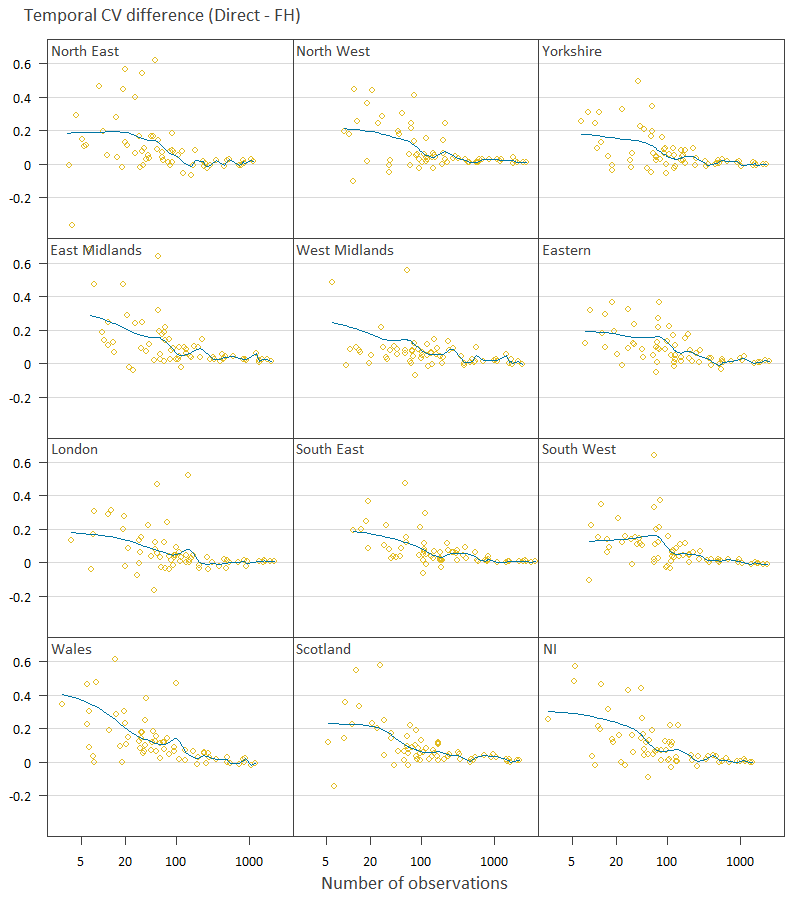
Source: Office for National Statistics
Notes:
Blue line is the trend.
Each point is a COICOP class.
Download this image Figure 11: Temporal coefficient of variation difference by sample size within each region, UK regions
.png (21.3 kB) .csv (15.5 kB)
Assessing the stability of the expenditure estimates derived from the LCF provides an incomplete picture of the benefits of SAE. The expenditure estimates still require adjustments based on balancing with other data sources before they can be used as expenditure weights for the regional CPI. The stability of the balanced expenditure estimates is important for the stability of the regional CPI. Ultimately we should assess the outcome through its impact on the regional CPIs, rather than on the unadjusted expenditure weights. Since the adjusted weights do not include all data sources, such as Council Tax, it is not completely accurate to call it the regional CPI. We emphasise that this “regional CPI” presented in this report is merely an experimental statistic at this stage of development, hence is not the exact regional analogue of the national CPI.
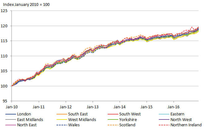
Before presenting the regional CPIs based on the adjusted estimates we first present the regional CPIs calculated with the national weights. This provides reference regional CPIs with verifiably stable weights. The differences between the regions will be understated since the only source of variation between regions comes from the prices.
Figure 12: Regional CPI using national expenditure weights, UK regions
Source: Office for National Statistics
Download this image Figure 12: Regional CPI using national expenditure weights, UK regions
.png (34.1 kB) .xls (47.1 kB)
Figure 12 shows the regional CPIs using the national expenditure weights. As expected there is not much difference between the regions and there are no unrealistically volatile movements over time.
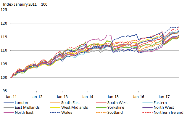
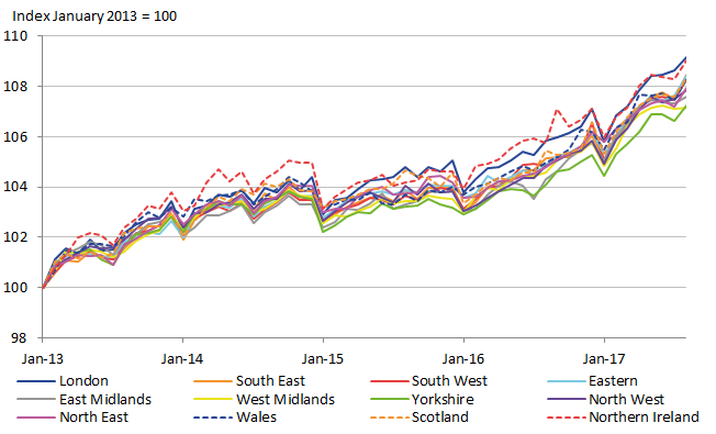
The regional CPIs generated with the adjusted direct estimate weights and the adjusted FH estimate weights are shown in Figure 13 and Figure 14 respectively. While there are noticeable differences, they both share large irregularities when the expenditure weights change at the new year. This is particularly noticeable in the latter years. However, there is a noticeable difference between the two figures, showing that the irregularities do appear to be lesser for the FH estimates. So the evidence of improved stability in the expenditure estimates is also being seen in the resulting regional CPIs.
Figure 13: Regional CPI using direct estimates, UK regions
Source: Office for National Statistics
Download this image Figure 13: Regional CPI using direct estimates, UK regions
.png (52.9 kB) .xls (57.9 kB)
Figure 14: Regional CPI using Fay-Herriot estimates, UK regions

Source: Office for National Statistics
Download this image Figure 14: Regional CPI using Fay-Herriot estimates, UK regions
.png (44.8 kB) .xls (46.6 kB)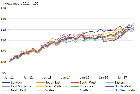
Although there do appear to be improvements in the stability of the regional CPI in Figure 14, it is still evident that this is not the stability that would be required of a reliable index. This can be seen by the erratic rising and falling in 2015 to 2017 when the year changes. These rises and falls are greater with the direct estimates, but nevertheless they are problematic in both. This suggests that FH estimates alone do not overcome the problem of temporal instability.
To further understand the instability in the regional CPIs we look further into the causes. To do this we identify and assess the COICOP classes with the least stable adjusted weights. For the North East, the most notably unstable classes are 4.5.1 “Electricity”, 8.2 “Telephone and telefax equipment and services”, 9.2.1 and 9.2.2 “Major durables for in and outdoor recreation” and 10.0 “Education”. Figures 15a and 15b shows the adjusted and unadjusted weights for these four classes. Recall that the unadjusted weights are calculated from the LCF expenditure estimates whereas the adjusted weights attempt to account for the other data sources, underreporting, and so on. There are two important features that this figure shows. First, the adjusted weights for these four classes are all unrealistically volatile over time, for example, for COICOP Class 8.2, 62ppt in 2016 falling to 13ppt in 2017. Secondly, the unadjusted weights are approximately six times smaller than the adjusted weights. These four COICOP classes all have small number of observations, as well as unadjusted relative expenditure all less than 1%, yet adjustment increases them substantially. This means that the adjustment process undertaken by ONS is magnifying the problem of small observation numbers. For example, consider COICOP Class 4.5.1, which had no observations in 2018 yet in previous years represents 2 to 4% of the basket.
Figure 15a: Adjusted weight for four particularly unstable COICOP classes, North East region
Source: Office for National Statistics
Notes:
- COICOP classes: Electricity = 4.5.1, Telephone equipment and services = 8.2, Major durables for recreation = 9.2.1, Education = 10.
Download this chart Figure 15a: Adjusted weight for four particularly unstable COICOP classes, North East region
Image .csv .xls
Figure 15b: Unadjusted weight for four particularly unstable COICOP classes, North East region
Source: Office for National Statistics
Notes:
- COICOP classes: Electricity = 4.5.1, Telephone equipment and services = 8.2, Major durables for recreation = 9.2.1, Education = 10.
Download this chart Figure 15b: Unadjusted weight for four particularly unstable COICOP classes, North East region
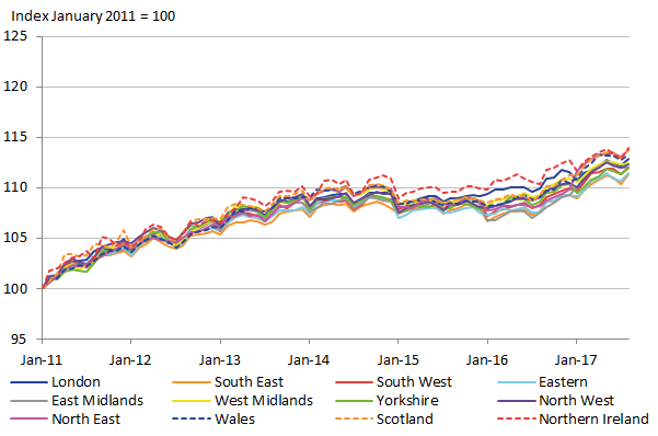
Image .csv .xlsTo appreciate the effect of these four classes alone on the volatility of the regional CPI, we present the regional CPI without these classes. If the volatility substantially diminishes then it is further proof that it is these COICOP classes causing significant instability to the CPI. The regional CPI with these classes removed is shown in Figure 16.
Figure 16: Regional CPI with Fay-Herriot estimates and four volatile COICOP classes (4.5.1, 8.2, 9.2.1/2 and 10.0) removed
Source: Office for National Statistics
Download this image Figure 16: Regional CPI with Fay-Herriot estimates and four volatile COICOP classes (4.5.1, 8.2, 9.2.1/2 and 10.0) removed
.png (32.4 kB) .xls (57.9 kB)
The volatility of the regional CPIs has clearly been substantially reduced. The regional CPIs without these four classes are comparable in smoothness to the regional CPIs with the national weights in Figure 12. This suggests that the temporal instability is mostly caused by just four COICOP classes, and these classes are all unstable due to the weights being inflated when adjusted.
While this diagnoses a significant cause of the problem of temporal volatility, we now assess whether smoothing methods can alleviate the problem.
Smoothing methods
Since initial attempts to reduce the volatility of the regional CPI through borrowing strength from other regions (using SAE) were not entirely successful for all classes, it may be that borrowing strength from other years is required. The primary aim is to reduce temporal instability, so methods that smooth over time should be able to further achieve. There are many smoothing methods which can be used, but for simplicity we test whether a three-year moving average of the expenditure weights substantially reduces the temporal instability. So instead of taking the mean estimate from observations in a given year, we include that year as well as the observations in the two preceding years. This serves to reduce the number of non-zero expenditure outcomes, as well as strengthen the temporal correlation.
To observe the effect that the three-year moving average has on reducing temporal instability, we present the regional CPIs in Figure 17. Note that the series of regional CPIs is two years shorter due to the averaging. Nevertheless, there is evidence of improved stability compared to the one-year direct estimates presented in Figure 13. However, there is still some remaining volatility in the regional CPIs, most notably for Wales in 2015. It seems that the three-year moving average approach does not eliminate all problems of volatility. Next, FH estimation was applied to the three-year moving average estimates, to observe the effect of both SAE and smoothing methods. The resulting regional CPIs are shown in Figure 18. It appears that there is no longer any clear unrealistic volatility in the indices, suggesting that a reliable method for producing regional CPI expenditure weights will rely on both SAE and smoothing methods together.
Figure 17: Regional CPI with expenditure weights using three-year moving average of direct estimates

Source: Office for National Statistics
Download this image Figure 17: Regional CPI with expenditure weights using three-year moving average of direct estimates
.png (46.1 kB) .xls (42.0 kB)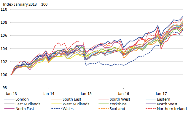
Figure 18: Regional CPI with expenditure weights using Fay-Herriot estimates on three-year moving averages
Source: Office for National Statistics
Download this image Figure 18: Regional CPI with expenditure weights using Fay-Herriot estimates on three-year moving averages
.png (52.9 kB) .xls (52.2 kB)
The results show that SAE methods using FH models for individual classes can improve the stability of the expenditure weights. The classes that benefit the most tended to have fewer than 100 observations, but also with enough observations for a good model to be fitted. FH models for regions with zero expenditure cause problems resulting in the model being unable to be fitted. Although FH models do improve the stability they do not lead to adjusted weights that provide stable regional CPIs.
One potential method for improving the SAE methods would be to use a multivariate FH model. This could be used to incorporate the correlation structure between the COICOP classes, and in doing so provide further stability to the estimates. For example, related classes like 1.1.2 “Meat” and 1.1.3 “Fish” may have an underlying correlation, which can be used in the model to improve the precision of the estimates. However, there are limitations with this multivariate approach.
The first limitation is that the correlations between the COICOP classes would need to be estimated, which would have the same difficulties with few observations. Second, the correlations between COICOP classes may be quite weak at the regional level and hence not offer much benefit. Thirdly, the multivariate FH approach requires complex computations which makes the approach difficult to implement, especially with large numbers of classes. This makes it probable that the model would be unable to converge on a solution, even with good correlation estimates. Due to these limitations we believe that the multivariate method will not offer worthwhile improvements.
Nôl i'r tabl cynnwys7. Summary and recommendations
We have assessed the extent that small area estimation (SAE) using Fay-Herriot (FH) models can be used to improve the temporal stability of expenditure estimates. First, we showed that using Living Costs and Food (LCF) survey observations classified at a higher level of Classification of Individual Consumption by Purpose (COICOP) increases the number of groups where SAE can be conducted. COICOP classes have more observations and higher expenditures, which reduces estimation problems caused by high numbers of zeroes. Then we showed the effects that FH models have on the estimates compared to the direct estimates. There was clear evidence of reduction in the coefficient of variation (CVs) in almost all cases, indicating that FH estimation was not merely making non-trivial differences in the estimates, except in classes with many observations. Classes with smaller numbers of observations benefited the most.
Although FH estimation improved temporal stability, the resulting regional Consumer Prices Index (CPIs) revealed that there was still enough instability to be problematic. A closer assessment showed that the instability was largely caused by four COICOP classes. These classes all had small unadjusted weights that had been increased by large factors of around six times during the balancing adjustments. This magnified the instability in the resulting regional CPIs.
Smoothing methods were briefly considered as another method of reducing temporal volatility. We showed that a three-year moving average reduces the instability, but not sufficiently to produce credible regional series. Combining smoothing methods as well as SAE did result in regional CPIs which appeared absent of unrealistic volatility.
We conclude that SAE does generally improve the stability of the expenditure weight estimates. However, it does not fully solve the problem. We identified particular COICOP classes that have unrealistic instability over time, and hence require more methods than just SAE. Furthermore, smoothing methods show evidence of being useful. Based on this we make the following recommendations:
the methods used for expenditure weight adjustment should be reviewed, identifying the causes of disparities between unadjusted and adjusted weights
review the additional data sources for COICOP classes that are strongly underrepresented in the LCF survey
from the first two points, undertake an investigation into estimation and smoothing techniques to be used in conjunction with multiple data sources
provide quality measures which a regional CPI or Consumer Prices Index, including owner occupiers’ housing costs (CPIH) should aim to achieve; this will help identify what is an acceptable level of temporal variability over time, comparisons to the national CPI or CPIH may be useful for this
develop methods which utilise the recently released regional household final consumption expenditure data
assess the temporal stability of the regional price quotes and the capacity for price estimation to be improved using model-based methods
References
Dawber, J and Smith, P.A. (2017) Feasibility study into producing CPIH consistent inflation rates for UK regions.
Rao, J. N., and Molina, I. (2015). Small area estimation (Second Edition). John Wiley and Sons.
8. Appendix
| North East | North West | Yorkshire and the Humber | East Midlands | West Midlands | East | London | South East | South West | Wales | Scotland | Northern Ireland | |
|---|---|---|---|---|---|---|---|---|---|---|---|---|
| 1.1.1 | 1086 | 2515 | 1965 | 1892 | 2023 | 2126 | 1664 | 3168 | 2041 | 907 | 1859 | 669 |
| 1.1.2 | 806 | 1871 | 1510 | 1458 | 1525 | 1684 | 1159 | 2424 | 1589 | 681 | 1386 | 555 |
| 1.1.3 | 237 | 567 | 425 | 441 | 470 | 544 | 469 | 789 | 496 | 183 | 400 | 116 |
| 1.1.4 | 854 | 2044 | 1565 | 1611 | 1692 | 1797 | 1440 | 2640 | 1731 | 733 | 1503 | 551 |
| 1.1.5 | 249 | 561 | 410 | 447 | 471 | 511 | 401 | 761 | 501 | 201 | 407 | 155 |
| 1.1.6 | 747 | 1789 | 1380 | 1471 | 1569 | 1683 | 1601 | 2648 | 1743 | 688 | 1396 | 498 |
| 1.1.7 | 1098 | 2640 | 2140 | 2104 | 2252 | 2393 | 1952 | 3543 | 2319 | 956 | 1946 | 697 |
| 1.1.8 | 529 | 1279 | 985 | 972 | 1051 | 1094 | 782 | 1574 | 1057 | 478 | 989 | 352 |
| 1.1.9 | 199 | 474 | 348 | 361 | 382 | 372 | 334 | 553 | 371 | 164 | 323 | 131 |
| 1.2.1 | 161 | 416 | 327 | 351 | 337 | 384 | 254 | 556 | 391 | 159 | 293 | 108 |
| 1.2.2 | 352 | 857 | 628 | 662 | 652 | 695 | 612 | 1010 | 655 | 289 | 664 | 242 |
| 2.1.1 | 33 | 93 | 87 | 70 | 60 | 62 | 60 | 119 | 65 | 23 | 97 | 22 |
| 2.1.2 | 118 | 321 | 222 | 234 | 232 | 292 | 183 | 439 | 282 | 119 | 231 | 68 |
| 2.1.3 | 68 | 150 | 118 | 116 | 108 | 129 | 78 | 191 | 112 | 51 | 96 | 35 |
| 2.2. | 51 | 148 | 105 | 105 | 100 | 105 | 61 | 150 | 117 | 45 | 107 | 41 |
| 3.1.2 | 291 | 649 | 538 | 446 | 526 | 550 | 401 | 833 | 529 | 253 | 471 | 230 |
| 3.1.3 | 39 | 101 | 86 | 91 | 91 | 99 | 74 | 142 | 86 | 49 | 81 | 38 |
| 3.1.4 | 4 | 15 | 8 | 15 | 11 | 18 | 29 | 29 | 11 | 6 | 8 | 4 |
| 3.2 | 82 | 186 | 164 | 138 | 144 | 148 | 125 | 191 | 132 | 66 | 111 | 75 |
| 4.1 | 0 | 1 | 2 | 0 | 0 | 1 | 0 | 0 | 0 | 0 | 1 | 0 |
| 4.2 | 0 | 0 | 0 | 0 | 0 | 0 | 0 | 0 | 0 | 0 | 0 | 0 |
| 4.3.1 | 44 | 84 | 65 | 87 | 53 | 70 | 32 | 115 | 74 | 27 | 59 | 18 |
| 4.3.2 | 0 | 0 | 0 | 0 | 0 | 0 | 0 | 0 | 0 | 0 | 0 | 0 |
| 4.4.1 | 0 | 0 | 0 | 0 | 2 | 0 | 0 | 0 | 0 | 0 | 0 | 0 |
| 4.4.3 | 0 | 0 | 0 | 0 | 0 | 0 | 0 | 0 | 0 | 0 | 0 | 0 |
| 4.5.1 | 0 | 1 | 0 | 2 | 1 | 0 | 0 | 3 | 2 | 0 | 2 | 1 |
| 4.5.2 | 0 | 1 | 1 | 3 | 1 | 2 | 0 | 5 | 5 | 0 | 2 | 0 |
| 4.5.3 | 0 | 0 | 0 | 1 | 1 | 1 | 0 | 0 | 0 | 2 | 0 | 1 |
| 4.5.4 | 5 | 16 | 13 | 9 | 11 | 11 | 3 | 13 | 14 | 11 | 8 | 12 |
| 4.9 | 0 | 0 | 0 | 0 | 0 | 0 | 0 | 0 | 0 | 0 | 0 | 0 |
| 5.1.1 | 38 | 92 | 68 | 72 | 70 | 77 | 43 | 116 | 56 | 41 | 62 | 18 |
| 5.1.2 | 3 | 4 | 6 | 7 | 6 | 1 | 2 | 4 | 5 | 2 | 4 | 2 |
| 5.2 | 53 | 122 | 89 | 97 | 96 | 113 | 65 | 161 | 93 | 57 | 95 | 35 |
| 5.3.1 | 19 | 57 | 39 | 38 | 38 | 37 | 26 | 54 | 36 | 17 | 30 | 7 |
| 5.3.3 | 1 | 3 | 5 | 5 | 2 | 7 | 2 | 7 | 4 | 2 | 5 | 5 |
| 5.4 | 95 | 213 | 169 | 185 | 178 | 198 | 154 | 323 | 176 | 97 | 160 | 50 |
| 5.5 | 83 | 252 | 158 | 189 | 148 | 201 | 127 | 315 | 203 | 77 | 144 | 49 |
| 5.6.1 | 463 | 1102 | 806 | 823 | 928 | 973 | 718 | 1487 | 918 | 466 | 830 | 312 |
| 5.6.2 | 47 | 112 | 96 | 60 | 69 | 78 | 50 | 96 | 61 | 19 | 71 | 50 |
| 6.1.1 | 106 | 267 | 221 | 204 | 219 | 239 | 167 | 380 | 219 | 94 | 175 | 59 |
| 6.1.2 | 46 | 117 | 85 | 70 | 63 | 92 | 61 | 127 | 76 | 21 | 61 | 15 |
| 6.2.1 | 5 | 14 | 17 | 10 | 16 | 21 | 16 | 37 | 32 | 2 | 14 | 4 |
| 6.2.2 | 6 | 19 | 21 | 16 | 13 | 39 | 14 | 57 | 32 | 6 | 16 | 4 |
| 6.3 | 0 | 0 | 1 | 0 | 1 | 0 | 0 | 0 | 0 | 0 | 0 | 0 |
| 7.1.1A | 20 | 33 | 18 | 9 | 22 | 28 | 8 | 36 | 24 | 6 | 25 | 2 |
| 7.1.1B | 25 | 42 | 47 | 51 | 33 | 41 | 18 | 56 | 36 | 15 | 41 | 6 |
| 7.1.2 | 2 | 4 | 3 | 5 | 3 | 4 | 4 | 5 | 3 | 2 | 4 | 2 |
| 7.2.1 | 27 | 70 | 62 | 53 | 57 | 67 | 33 | 119 | 57 | 34 | 63 | 24 |
| 7.2.2 | 168 | 417 | 332 | 343 | 357 | 396 | 232 | 600 | 377 | 174 | 309 | 127 |
| 7.2.3 | 28 | 106 | 84 | 77 | 71 | 114 | 60 | 195 | 121 | 34 | 48 | 14 |
| 7.2.4 | 55 | 124 | 95 | 116 | 117 | 150 | 86 | 231 | 145 | 47 | 69 | 33 |
| 7.3.1 | 23 | 61 | 52 | 36 | 47 | 59 | 84 | 127 | 35 | 14 | 56 | 4 |
| 7.3.2 | 91 | 165 | 182 | 119 | 100 | 103 | 79 | 148 | 75 | 55 | 123 | 56 |
| 7.3.3 | 1 | 8 | 4 | 4 | 0 | 6 | 12 | 6 | 5 | 3 | 3 | 2 |
| 7.3.4 | 1 | 1 | 0 | 3 | 4 | 2 | 3 | 12 | 6 | 0 | 2 | 0 |
| 8.1 | 24 | 80 | 57 | 58 | 44 | 76 | 46 | 115 | 64 | 30 | 59 | 15 |
| 8.2 | 23 | 70 | 63 | 58 | 64 | 46 | 46 | 82 | 44 | 30 | 54 | 24 |
| 9.1.1 | 19 | 31 | 23 | 23 | 25 | 30 | 28 | 45 | 25 | 10 | 23 | 9 |
| 9.1.2 | 3 | 10 | 2 | 5 | 4 | 5 | 2 | 12 | 5 | 3 | 5 | 2 |
| 9.1.3 | 10 | 35 | 34 | 36 | 20 | 39 | 35 | 62 | 31 | 15 | 37 | 13 |
| 9.1.4 | 15 | 45 | 28 | 19 | 35 | 34 | 27 | 51 | 27 | 11 | 19 | 12 |
| 9.1.5 | 0 | 1 | 2 | 1 | 2 | 2 | 3 | 5 | 4 | 0 | 1 | 0 |
| 9.2.1 | 2 | 9 | 7 | 4 | 7 | 5 | 2 | 11 | 9 | 2 | 6 | 3 |
| 9.3.1 | 72 | 192 | 141 | 151 | 149 | 152 | 122 | 259 | 150 | 64 | 135 | 47 |
| 9.3.2 | 21 | 51 | 31 | 31 | 36 | 44 | 15 | 55 | 40 | 18 | 36 | 22 |
| 9.3.3 | 84 | 209 | 171 | 161 | 160 | 198 | 123 | 297 | 213 | 87 | 155 | 37 |
| 9.3.4 | 128 | 322 | 232 | 253 | 264 | 270 | 129 | 413 | 276 | 120 | 214 | 64 |
| 9.4.1 | 80 | 199 | 160 | 126 | 125 | 185 | 126 | 268 | 155 | 65 | 142 | 59 |
| 9.4.2 | 103 | 246 | 177 | 222 | 182 | 274 | 195 | 403 | 257 | 85 | 174 | 67 |
| 9.5.1 | 39 | 100 | 78 | 81 | 77 | 105 | 83 | 162 | 105 | 36 | 81 | 28 |
| 9.5.2 | 184 | 469 | 353 | 334 | 343 | 446 | 249 | 583 | 405 | 155 | 416 | 157 |
| 9.5.3 | 146 | 371 | 308 | 324 | 308 | 361 | 231 | 554 | 316 | 134 | 280 | 105 |
| 9.6 | 0 | 0 | 0 | 0 | 0 | 0 | 0 | 0 | 0 | 0 | 0 | 0 |
| 10 | 4 | 10 | 9 | 16 | 12 | 12 | 16 | 14 | 5 | 5 | 9 | 4 |
| 11.1.1 | 984 | 2140 | 1886 | 1515 | 1528 | 1782 | 1558 | 2557 | 1569 | 768 | 1549 | 691 |
| 11.1.2 | 61 | 120 | 100 | 94 | 95 | 107 | 99 | 161 | 76 | 47 | 111 | 36 |
| 11.2 | 2 | 3 | 3 | 2 | 1 | 0 | 3 | 4 | 1 | 1 | 2 | 0 |
| 12.1.1 | 59 | 134 | 115 | 111 | 97 | 132 | 92 | 185 | 118 | 36 | 102 | 54 |
| 12.1.2 | 5 | 9 | 17 | 9 | 11 | 14 | 5 | 16 | 10 | 3 | 6 | 4 |
| 12.3.1 | 31 | 67 | 48 | 61 | 48 | 60 | 40 | 82 | 47 | 29 | 52 | 23 |
| 12.3.2 | 35 | 98 | 77 | 70 | 72 | 83 | 53 | 125 | 67 | 27 | 55 | 22 |
| 12.4 | 9 | 26 | 23 | 24 | 36 | 26 | 23 | 37 | 23 | 6 | 21 | 12 |
| 12.5.2 | 5 | 14 | 9 | 15 | 13 | 15 | 8 | 24 | 18 | 7 | 8 | 0 |
| 12.5.3 | 0 | 4 | 3 | 4 | 0 | 6 | 1 | 1 | 0 | 0 | 0 | 1 |
| 12.5.4 | 3 | 6 | 5 | 0 | 2 | 3 | 4 | 13 | 6 | 3 | 4 | 0 |
| 12.6.2 | 1 | 0 | 0 | 2 | 0 | 0 | 2 | 1 | 0 | 0 | 0 | 0 |
| 12.7 | 32 | 98 | 84 | 78 | 46 | 62 | 55 | 115 | 56 | 27 | 44 | 31 |
Download this table Table 4: Number of observations for each Classification of Individual Consumption by Purpose (COICOP) class recorded in the 2014 Living Costs and Food (LCF) data
.xls .csv
| Too few observations (for Fay-Herriot estimation) | Many observations (> 100) | Negligible ppt (ppt < 0.5) | Negligible improvement in stability (median CV difference < 0.03) | Strong benefit for Fay-Herriot estimate | |
|---|---|---|---|---|---|
| 1.1.1 Bread and cereals | Yes | Yes | |||
| 1.1.2 Meat | Yes | Yes | |||
| 1.1.3 Fish | Yes | Yes | |||
| 1.1.4 Milk, cheese and eggs | Yes | Yes | |||
| 1.1.5 Oils and fats | Yes | Yes | |||
| 1.1.6 Fruit | Yes | Yes | |||
| 1.1.7 Vegetables including potatoes and tubers | Yes | Yes | |||
| 1.1.8 Sugar, jam, syrups, chocolate and confectionery | Yes | Yes | |||
| 1.1.9 Food products (nec) | Yes | Yes | |||
| 1.2.1 Coffee, tea and cocoa | Yes | Yes | |||
| 1.2.2 Mineral waters, soft drinks and juices | Yes | Yes | |||
| 2.1.1 Spirits | Yes | ||||
| 2.1.2 Wine | Yes | ||||
| 2.1.3 Beer | Yes | ||||
| 2.2 Tobacco | Yes | ||||
| 3.1.2 Garments | Yes | Yes | |||
| 3.1.3 Other clothing and clothing accessories | Yes | ||||
| 3.1.4 Cleaning, repair and hire of clothing | Yes | ||||
| 3.2 Footwear including repairs | Yes | ||||
| 4.1 Actual rentals for housing | Yes | Yes | |||
| 4.2 Owner occupiers' housing costs | Yes | Yes | |||
| 4.3.1 Materials for maintenance and repair | Yes | ||||
| 4.3.2 Services for maintenance and repair | Yes | Yes | |||
| 4.4.1 Water supply | Yes | Yes | |||
| 4.4.3 Sewerage collection | Yes | Yes | |||
| 4.5.1 Electricity | Yes | ||||
| 4.5.2 Gas | Yes | ||||
| 4.5.3 Liquid fuels | Yes | Yes | |||
| 4.5.4 Solid fuels | Yes | ||||
| 4.9 Council Tax and rates | Yes | Yes | |||
| 5.1.1 Furniture and furnishings | Yes | ||||
| 5.1.2 Carpets and other floor coverings | Yes | Yes | |||
| 5.2 Household textiles | Yes | ||||
| 5.3.1/2 Major appliances and small electric goods | Yes | ||||
| 5.3.3 Repair of household appliances | Yes | ||||
| 5.4 Glassware, tableware and household utensils | Yes | ||||
| 5.5 Tools and equipment for house and garden | Yes | ||||
| 5.6.1 Non-durable household goods | Yes | Yes | |||
| 5.6.2 Domestic services and household services | Yes | ||||
| 6.1.1 Pharmaceutical products | Yes | ||||
| 6.1.2/3 Other medical and therapeutic equipment | Yes | ||||
| 6.2.1/3 Medical services & paramedical services | Yes | ||||
| 6.2.2 Dental services | Yes | ||||
| 6.3 Hospital services | Yes | Yes | |||
| 7.1.2/3 Motorcycles and bicycles | Yes | ||||
| 7.1.1A New cars | Yes | ||||
| 7.1.1B Second-hand cars | Yes | Yes | |||
| 7.2.1 Spare parts and accessories | Yes | ||||
| 7.2.2 Fuels and lubricants | Yes | Yes | |||
| 7.2.3 Maintenance and repairs | Yes | ||||
| 7.2.4 Other services | Yes | ||||
| 7.3.1 Passenger transport by railway | Yes | ||||
| 7.3.2/6 Passenger transport by road and other transport services | Yes | ||||
| 7.3.3 Passenger transport by air | Yes | ||||
| 7.3.4 Passenger transport by sea and inland waterway | Yes | Yes | |||
| 8.1 Postal services | Yes | ||||
| 8.2/3 Telephone and telefax equipment and services | Yes | ||||
| 9.1.1 Reception and reproduction of sound and pictures | Yes | ||||
| 9.1.2 Photographic, cinematographic and optical equipment | Yes | ||||
| 9.1.3 Data processing equipment | Yes | ||||
| 9.1.4 Recording media | Yes | ||||
| 9.1.5 Repair of audio-visual equipment & related products | Yes | Yes | |||
| 9.2.1/2/3 Major durables for in/outdoor recreation | Yes | ||||
| 9.3.1 Games, toys and hobbies | Yes | ||||
| 9.3.2 Equipment for sport and open-air recreation | Yes | ||||
| 9.3.3 Gardens, plants and flowers | Yes | ||||
| 9.3.4/5 Pets, related products and services | Yes | ||||
| 9.4.1 Recreational and sporting services | Yes | ||||
| 9.4.2 Cultural services | Yes | ||||
| 9.5.1 Books | Yes | ||||
| 9.5.2 Newspapers and periodicals | Yes | Yes | |||
| 9.5.3/4 Misc. printed matter, stationery, drawing materials | Yes | Yes | |||
| 9.6 Package holidays | Yes | Yes | |||
| 10.0 Education | Yes | ||||
| 11.1.1 Restaurants & cafes | Yes | Yes | |||
| 11.1.2 Canteens | |||||
| 11.2 Accommodation services | Yes | Yes | |||
| 12.1.1 Hairdressing and personal grooming establishments | Yes | ||||
| 12.1.2/3 Appliances and products for personal care | Yes | Yes | |||
| 12.3.1 Jewellery, clocks and watches | Yes | ||||
| 12.3.2 Other personal effects | Yes | ||||
| 12.4 Social protection | Yes | ||||
| 12.5.2 House contents insurance | Yes | ||||
| 12.5.3/5 Health insurance and other insurance | Yes | Yes | |||
| 12.5.4 Transport insurance | Yes | Yes | |||
| 12.6.2 Other financial services | Yes | Yes | |||
| 12.7 Other services | Yes | ||||
| Total count | 21 | 22 | 19 | 22 | 37 |