1. Main points
- This article incorporates improvements to the methodology and data sources used for these statistics, including an upgrade to our statistical production system.
- Owner occupiers’ housing costs (OOH) in the UK under the rental equivalence approach have grown by 1.1% over the 12 months to September 2019.
- After incorporating the improvements, OOH according to the net acquisitions approach have grown by 1.6% over the 12 months to September 2019.
- After incorporating the improvements, OOH compiled using the payments approach have grown by 3.1% over the 12 months to September 2019.
2. Things you need to know about this release
Owner occupiers’ housing costs (OOH) are the costs of housing services associated with owning, maintaining and living in one’s own home. This is distinct from the cost of purchasing a house, which is purchased partly for the accumulation of wealth and partly for housing services.
OOH is an important component of the household consumption basket. In the Consumer Prices Index including owner occupiers’ housing costs (CPIH), the OOH component is measured using the rental equivalence approach, OOH(RE). However, there are other approaches to measuring OOH.
In this article, we focus on two alternative approaches: payments, OOH(payments) and net acquisitions, OOH(NA). The OOH(payments) approach is also used in a new set of indices called the Household Costs Indices, which aim to reflect changing prices and costs as experienced by households. This article compares these approaches to the rental equivalence approach and discusses the performance of the different measures over time, in prevailing economic conditions.
This article introduces several improvements to the way we calculate and publish the net acquisitions and payments approaches. In particular, the following improvements have been introduced:
- the development of a new methodology using new data sources for producing the Stamp Duty Index; this affects both the OOH(payments) and OOH(NA) series
- the development of a new statistical production system; we have used this as an opportunity to incorporate revisions in the national accounts expenditure data into the weights, and to correct some minor historical inaccuracies in the previous methodology
- the time series for OOH(payments) and OOH(NA) will now be published with monthly periodicity; previously the data were aggregated to a quarterly average time series before publishing
Section 3 presents results incorporating these improvements. This section also includes some analysis showing the impact of incorporating these approaches alongside the other components of our Consumer Prices Index (CPI) to calculate hybrid aggregate measures, CPI-H(payments) and CPI-H(NA). Section 4 explains the changes in more detail, in particular, the changes to Stamp Duty. The impact of these changes on the different measures of OOH are discussed in Section 5.
The first article in the series provides more information about the different approaches to measuring OOH to aid your understanding of the differences in concept, underlying methodology and data sources, and associated advantages and limitations to each approach. There have also been several “Spotlight” sections produced, which focus on different topics relating to OOH. These topics are listed in the “Related links” section.
You should note that the payments and net acquisitions approaches are both experimental indices and therefore we would caution against any use other than for research purposes. More information on the methodology for each approach can also be found in the CPIH compendium.
We are currently undergoing a review of our Prices publications. This could result in changes to the scheduling of OOH releases in the future.
There have been several improvements made within this release. We invite you to submit feedback on these changes and anything else related to this release to cpi@ons.gov.uk.
Nôl i'r tabl cynnwys3. Results
All results presented in this section incorporate the improvements discussed in Section 2, notably the introduction of new methodology to calculate the Stamp Duty Index and the incorporation of revisions in the national accounts expenditure data. The impacts of these changes are discussed in Section 5.
Figure 1 presents the cumulative indices for each approach and Figure 2 shows the annual growth rates. The index for the owner occupiers’ housing costs net acquisitions approach – OOH(NA) – has shown the strongest growth over the period (Figure 1). The payments approach – OOH(payments) – saw strong growth prior to the economic downturn in 2008 to 2009. However, of the three measures, it has also seen the largest fall since the economic downturn and has still not recovered its pre-downturn peak.
Over the period, the rental equivalence approach – OOH(RE) – experienced the fewest fluctuations in the 12-month growth rate (Figure 2). The growth rate of OOH(RE) was 1.1% in the 12 months to September 2019, compared with 3.1% for OOH(payments) and 1.6% for OOH(NA).
Figure 1: The index for the net acquisitions approach – OOH(NA) – has shown the strongest growth over the period since 2005
UK, Jan 2005 to Sep 2019
Source: Office for National Statistics
Download this chart Figure 1: The index for the net acquisitions approach – OOH(NA) – has shown the strongest growth over the period since 2005
Image .csv .xls
Figure 2: OOH(payments) has shown the fastest annual growth out of the three approaches since August 2018
UK, Jan 2006 to Sept 2019
Source: Office for National Statistics - Consumer price inflation
Download this chart Figure 2: OOH(payments) has shown the fastest annual growth out of the three approaches since August 2018
Image .csv .xlsFigure 3 presents the cumulative indices for each approach referenced at April 2009 to illustrate the change in each index from the lowest point of the economic downturn.
In the period shown, both OOH(NA) and OOH(payments) show stronger growth than OOH(RE). OOH(payments) was showing the strongest growth in the period up to December 2014, where from that period onwards, OOH(NA) took an upturn and has since exhibited the strongest growth up to the present period, September 2019. The primary reason for this is that mortgage interest rates and Stamp Duty, feeding into OOH(payments), have both experienced some decline over the period, whereas the price of new dwellings, feeding into OOH(NA), has experienced consistent growth over the same period.
Figure 3: Since the start of the recovery period from the 2008 economic downturn both OOH(NA) and OOH(Payments) have shown stronger growth than OOH(RE)
UK, Apr 2009 to Sept 2019
Source: Office for National Statistics - Consumer price inflation
Download this chart Figure 3: Since the start of the recovery period from the 2008 economic downturn both OOH(NA) and OOH(Payments) have shown stronger growth than OOH(RE)
Image .csv .xlsLooking at the contributions to growth can provide more insight into these trends. Figure 4 and Figure 5 present the contributions to the annual growth rate of OOH(NA) and OOH(payments) respectively, from the sub-indices used in their construction.
Because of the methodology used to calculate the owner occupiers’ housing costs rental equivalence approach – OOH(RE) – it is not possible to present a contributions chart for this approach. This is mainly because OOH(RE) is not constructed using a set of sub-indices that measure different concepts (for example, maintenance costs and Stamp Duty), but instead is aggregated from indices measuring the same concept across regions and tenure type.
“New dwellings”, “other services related to the acquisition of dwellings”, and “major repair and maintenance” explain most of the changes in the 12-month OOH(NA) price growth (Figure 5). The strong growth in the period leading up to the start of the economic downturn in 2008 is mainly driven by increases in the prices of new dwellings and other services related to the acquisition of dwellings. The “new dwellings” series uses the Office for National Statistics (ONS) House Price Index (HPI) as a proxy for change in the cost of new dwellings. Therefore, strong growth leading up to the start of the economic downturn can be explained by the growth experienced over the same period by UK house prices. The input data for “other services related to the acquisition of dwellings” is a combination of price indices for transfer costs and Stamp Duty.
New dwellings had a relatively strong negative contribution in the period October 2008 to December 2009, mirrored by the other services related to the acquisition of dwellings. This was likely caused by shrinking demand for housing resulting from the economic downturn, which in turn affected both house prices and transfer costs (including Stamp Duty).
In the period following the recovery, growth in OOH(NA) was again driven by new dwellings and other services related to the acquisition of dwellings. House prices fell again in the period 2010 to 2013, corresponding to the second dip in the series. The two dips in the “other services related to the acquisition of dwellings” beginning in December 2015 and December 2018 relate to changes in Stamp Duty discussed further in Section 4.
Figure 4: On average the new dwellings component is the largest contributor to owner occupiers’ housing costs net acquisitions - OOH(NA) - growth in the period since January 2005
UK, Jan 2006 to Sept 2019
Source: Office for National Statistics - Consumer price inflation
Download this chart Figure 4: On average the new dwellings component is the largest contributor to owner occupiers’ housing costs net acquisitions - OOH(NA) - growth in the period since January 2005
Image .csv .xlsFor the payments approach, it is the sub-index for mortgage interest payments that has the greatest impact on the aggregate series (Figure 5). Prior to the economic downturn in 2008, mortgage interest payments contributed positively to the growth of OOH(payments), which peaked in August 2007. This can be explained by growth in the Bank of England base rate from 3.5% in July 2003 to 5.75% in July 2007. As the economic downturn took hold and the Bank of England responded to the financial market shock, the base rate fell to a historic low of 0.5% in March 2009. The corresponding decline can be seen in the negative contributions from mortgage interest payments, which drove the dramatic fall in the OOH(payments) annual growth rate in 2009.
Since the beginning of 2012, OOH(payments) has seen less volatile growth compared with the period leading up to and directly after the economic downturn. The introduction of marginal tax rates for Stamp Duty in December 2014 (explained in Section 4, Changes to the Stamp Duty Index methodology) led to a fall in the overall OOH(payments) index in 2015.
Changes to the base rate in August 2016 (from 0.5% to 0.25%) resulted in negative contributions from mortgage interest payments during 2017. Subsequent increases in the base rate (from 0.25% to 0.5% in October 2017 and from 0.5% to 0.75% in August 2018) have led to increasing contributions from mortgage interest payments, offset by changes to the Stamp Duty tax rate discussed in Section 4.
Figure 5: Mortgage interest rates is the largest contributor to owner occupiers’ housing costs payments - OOH(Payments) - growth in the period since January 2005
UK, Jan 2006 to Sept 2019
Source: Office for National Statistics - Consumer price inflation
Download this chart Figure 5: Mortgage interest rates is the largest contributor to owner occupiers’ housing costs payments - OOH(Payments) - growth in the period since January 2005
Image .csv .xlsEach of these experimental approaches can be aggregated with the Consumer Prices Index (CPI), to create a hybrid aggregate inflation measure that includes OOH. These are known as CPI-H(payments) and CPI-H(NA).
Figure 6 presents the cumulative indices for each approach compared with the headline CPIH (which uses the rental equivalence approach) and Figure 7 shows the annual growth rates for these three indices. For more information about the three approaches, including the strengths and limitations of each approach and why the rental equivalence approach is our preferred measure, please see the CPIH compendium.
CPI-H(NA) appears to be heavily influenced by movements in house prices, falling faster compared with CPIH in the immediate aftermath of the economic downturn and growing faster afterwards during the recovery of the housing market. CPI-H(payments) exhibits similar movements but on a more substantial scale, demonstrating the impact of mortgage interest payments on the indices. In particular, the reduction of the Bank of England base rate in 2009 caused the growth of CPI-H(payments) to turn negative in April 2009.
In the period from 2005 to 2011, the average difference in the annual growth rate for the three measures was quite significant, at 0.9 percentage points. However, over the period since January 2012, all three measures have experienced similar rates of annual growth, with the average difference being 0.2 percentage points.
Figure 6: Over the period since 2005, CPI-H(NA) has experienced the highest rate of growth
UK, Jan 2005 to Sept 2019
Source: Office for National Statistics - Consumer price inflation
Download this chart Figure 6: Over the period since 2005, CPI-H(NA) has experienced the highest rate of growth
Image .csv .xls
Figure 7: The aggregate measures have experienced similar rates of annual growth over the period since 2012
UK, Jan 2006 to Sept 2019
Source: Office for National Statistics - Consumer price inflation
Download this chart Figure 7: The aggregate measures have experienced similar rates of annual growth over the period since 2012
Image .csv .xls4. Improvements to production
Revisions to OOH(NA) and OOH(payments) expenditure weights
The data sources for sub-indices expenditure weights for the owner occupiers’ housing costs net acquisitions approach – (OOH(NA)) and OOH(payments) are given in Table 1 and Table 2 respectively. Both series use data from the national accounts gross fixed capital formation (GFCF) and the household final consumption expenditure (HHFCE) data for certain components.
| Acquisition of dwellings | Ownership of dwellings | |||||
|---|---|---|---|---|---|---|
| OOH(NA) indices | Acquisitions of new dwellings (exc. Land) | Self builds and renovations | Existing dwellings new to the OOH sector | Services related to acquisition | Major repairs and maintenance | Insurance connected with the dwelling |
| Source of weights data | GFCF | GFCF | No weight currently exists | HHFCE and GFCF | HHFCE | HHFCE |
Download this table Table 1: Source data for OOH(NA) sub-indices weights
.xls .csv
| OOH(RE) Indices | Mortgage interest payments | Dwelling insurance | Ground rent | Stamp Duty | Estate agent fees | Home-buyers survey | Major repairs and maintenance | House conveyancing |
|---|---|---|---|---|---|---|---|---|
| Source of weights data | RPI | RPI | RPI | HHFCE and GFCF | RPI | RPI | HHFCE | RPI |
Download this table Table 2: Source data for OOH(Payments) sub-indices weights
.xls .csvThe GFCF and HHFCE data are taken from the latest available national accounts dataset, which is consistent with the most recent Blue Book release (typically published between June and October each year). Thus, for a given year y, the expenditure weights are based on the Blue Book release y-1, which publishes data for y-2. As an example, the expenditure weights for the year 2020 are based on the Blue Book release from October 2019, which publishes data for 2018.
National accounts estimates are open for revisions and therefore there can be differences between the initial expenditure estimates used to calculate OOH weights and revised expenditure totals for each year provided in subsequent Blue Book releases. Sometimes changes to data sources and the methodology from which the Blue Book is compiled results in a significant change to the revised back series of expenditure totals. These changes were previously noted and explained in the Spotlight section on the Revisions to OOH(RE) expenditure weights, up to the Blue Book 2016 release.
While the Consumer Prices Index including owner occupiers’ housing costs (CPIH) is very rarely revised because of consistency with the revisions policy for Consumer Prices Index (CPI) and Retail Prices Index (RPI), the net acquisitions and payments approaches are still experimental. This means that these indices can be revised where it is deemed a quality improvement. An improvement to the statistical production system provides the opportunity to recalculate the back series with significantly less effort, and so a decision to update both the OOH(payments) and OOH(NA) index series using the latest available expenditure data was made.
The national accounts revisions will likely impact the OOH(NA) index more than the OOH(payments) index because of five out of the six sub-indices weights for OOH(NA) being dependent on national accounts data, compared with two out of the eight (Stamp Duty, and major repairs and maintenance) for OOH(payments). The effects of these impacts are discussed in Section 5.
Changes to the Stamp Duty Index methodology
The price of Stamp Duty is a contributor to both the net acquisitions method (aggregated together with transfer costs to form “1.1.1.3. Other services related to the acquisition of dwellings”), and the payments method.
The growth in the Stamp Duty Index is affected by two factors:
- the rise and fall in property prices (the value on which the tax is paid)
- the current tax rules in place for the region in which the property was sold
There are different sets of rules in place across the regions of England, and Northern Ireland, Scotland and Wales. The use of the terms “Stamp Duty” and “Stamp Duty Index” in the analysis section refer to all three tax types in the following list:
- Stamp Duty Land Tax (SDLT) – covering England and Northern Ireland
- Land and Buildings Transaction Tax (LBTT) – covering Scotland
- Land Transaction Tax (LTT) – covering Wales
Further information on each can be found on the relevant government websites linked in the list.
Background
The method by which Stamp Duty Land Tax (SDLT) is charged to property buyers has changed a lot over the last 15 years. New governments bring in new tax rates, change existing tax rates and alter the thresholds at which different rates are applied. Figure 8 provides a summary timeline of the changes introduced.
From 3 December 2014, Stamp Duty underwent a significant change. New rules were brought in so that Stamp Duty was now only payable on the portion of the value of the tax bracket that it falls into, similarly to the way Income Tax is collected. That is, it changed from an “effective” tax rate, to a “marginal” tax rate.
This was closely followed by a devolution of powers to the Scottish Government, allowing them to set their own rules on tax rates and thresholds. This gave rise to the Land and Buildings Transaction Tax (LBTT), which now applies across Scotland. More recently, at the start of April 2018, the Welsh Government created a new tax for property transactions in Wales, the Land Transaction Tax (LTT).
There have also been a few noteworthy Stamp Duty tax “reliefs” or “holidays” in the recent past:
- as a response to the economic downturn caused by the global banking crisis in 2008, a Stamp Duty holiday for the basic threshold started on 3 September 2008, in which the basic threshold was raised £50,000 from £125,000 to £175,000; this ended on 31 December 2009
- a first-time buyer (FTB) rate was introduced by then Chancellor Alistair Darling on 25 March 2010, in which first-time-buyers enjoyed a 0% rate for properties up to a value of £250,000; this was taken away from 1 January 2012
- on 22 November 2017, first-time buyer relief returned for England, Wales and Northern Ireland; this time, first-time buyers would pay no tax on the value of a property up to £300,000 and then 5% for the portion between £300,001 and £500,000; if the property exceeds £500,000, then the standard rates apply on the entire price
- the Scottish Government followed suit on 1 July 2018, introducing a first-time buyers’ relief on LBTT, resulting in a 0% tax rate on the portion of the property under £175,000, as opposed to the threshold of £145,000 for non-first-time buyers
- the introduction of the LTT by the Welsh Government in April 2018 removed the application of first-time buyers’ relief across Wales
Figure 8: Summary timeline of stamp duty tax changes over the period 2005 to 2020
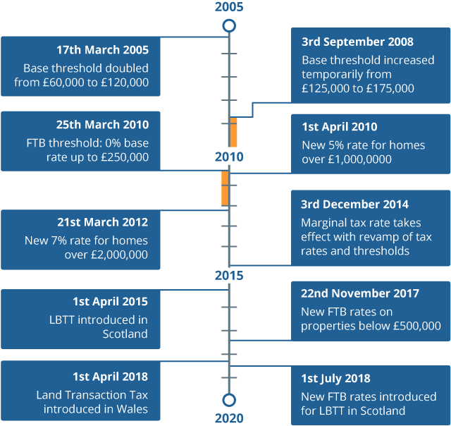
Source: Office for National Statistics
Notes:
- The two orange bars represent the start and end of the temporary rules (starting at their base).
Download this image Figure 8: Summary timeline of stamp duty tax changes over the period 2005 to 2020
.png (49.6 kB)
Previous methodology
The method used previously to calculate an estimate of the Stamp Duty Index relied on using averaged house price data and the number of sales within arbitrary house price bands.
The previous methodology for producing the Stamp Duty Index can be described in the following steps:
- using HM Land Registry price paid data for housing transactions, take the number of sales per price band during the base period (Quarter 4 (Oct to Dec) of the previous year, Q4y-1)
- uprate the number of sales for each month by using the within-year House Price Index (HPI) for the UK (lagged by one month); this results in a percentage of housing transactions moving into a higher or lower house price band
- for each house price band, calculate the expected Stamp Duty yield per transaction within the band (using the midpoint value) and multiply that by the number of houses within the band
- sum the total expected Stamp Duty yield for each month, to calculate a fixed quantity Stamp Duty yield from which the index is calculated
The method of using arbitrary house price bands to group property transaction prices resulted in several assumptions needing to be made in order to reach an estimate. For example, a uniform distribution of sales within price bands was assumed and the average price of all transactions within the band was assumed to be the midpoint. Furthermore, uprating the number of sales by the UK HPI meant that potentially important regional effects on the price of Stamp Duty were not being captured by the index.
New data sources
Recent improvements to the statistical production system used to calculate the OOH index opened the door to use more granular data sources in the calculation of the Stamp Duty Index. These new data consisted of final residential property transaction prices across England, Scotland and Wales, with each individual transaction price having been uprated month-by-month by the House Price Index at the local authority level.
The sources for the price data are HM Land Registry for England and Wales who provide residential property transactions for England and Wales, and Registers of Scotland (RoS) who provide residential property sales for Scotland. Individual residential property sales for Northern Ireland are not provided by the Northern Ireland Statistics and Research Agency – instead they compile the Northern Ireland House Price Index, which is then provided to the Office for National Statistics (ONS) on a quarterly basis and combined with Great Britain data to give overall figures for the UK. Therefore, the new method does not include any Stamp Duty contributions from Northern Ireland. In the period 2018 to 2019, Stamp Duty receipts from Northern Ireland accounted for only 0.7% of total receipts so their impact on the outcome of the Stamp Duty Index would most likely be negligible.
A metadata column describing the buyer status (for example, first-time or former owner-occupier) is also available in the dataset from 2012 onwards. This has been produced by matching data from the Council of Mortgage Lenders with data from HM Land Registry and Registers of Scotland, followed by an imputation. This will, by definition, not cover cash purchases. For these, it is assumed that they are all purchases by former owner-occupiers. For these reasons the metadata column is described as experimental and therefore we would caution against any use other than for research purposes. However, it provides an opportunity to capture the effect that first-time buyers’ relief has on the Stamp Duty Index.
A more comprehensive description of the methodology and data sources used to produce this dataset is described in the UK House Price Index quality and methodology guidance on GOV.UK.
New methodology
With the monthly uprating of prices for a fixed sample of houses already taken care of in the new data source, the methodology to calculate the Stamp Duty Index can be broadly simplified to:
- calculate the Stamp Duty yield for each monthly uprated transaction price
- sum the total Stamp Duty yield for each month to get the fixed quantity Stamp Duty yield
- calculate the index by dividing by the total yield from the base period
The method for calculating the Stamp Duty yield in step 1 is dependent on three variables within the data:
- the region in which the transaction was recorded
- the monthly period (in which the price has been uprated to)
- the buyer status (whether they are first-time or a former owner-occupier)
These variables are used to determine:
- which devolved tax type applies (SDLT, LTT or LBTT)
- which rules were in place for that tax type for the month in question
- what tax relief was applicable for first-time buyers
Any changes to the tax rules for calculating the various types of Stamp Duty (SDLT, LTT and LBTT), come into effect on a certain date. An arbitrary threshold has been applied to determine which month new rules apply on, depending on the day of the month in which they are introduced. Any tax changes coming into effect on or before the 14th of the month will apply to prices within the month in question. Any changes brought in after that date apply to the following month.
There have been two equations used in the calculation of Stamp Duty for the period observed. The first is for the effective tax rate (applicable pre-3 December 2014) and the other is for the marginal tax rate (applicable from 3 December 2014).
Both equations require a set of corresponding price thresholds and tax rates as a percentage, which govern the variables used within each equation. As an example, the current tax rates and thresholds for Stamp Duty Land Tax applying to former owner-occupiers in England and Northern Ireland (at the time of writing) are given in Table 3.
| Property or lease premium or transfer value | SDLT rate |
|---|---|
| Up to £125,000 | Zero |
| The next £125,000 (the portion from £125,001 to £250,000) | 2% |
| The next £675,000 (the portion from £250,001 to £925,000) | 5% |
| The next £575,000 (the portion from £925,001 to £1.5 million) | 10% |
| The remaining amount (the portion above £1.5 million) | 12% |
Download this table Table 3: Stamp Duty Land Tax rates if you have bought a home before
.xls .csvThe effective tax rate for Stamp Duty for an individual property is given by the following equation:
Where:
taxrateti is the tax rate applicable to the ith tax tier, t
price is the transaction price of the property, and
i is given by the tax tier that the price falls within
The equation for the marginal tax rate is:
where the additional terms are:
minthreshti is the minimum threshold applicable to the ith tax tier, t
maxthreshtj is the maximum threshold applicable to the jth tax tier, t
is the sum of all tax tiers up to the ith tax tier
The following worked example for a property sold at £625,000 demonstrates how the marginal tax rate works in practice. It uses the tax rates and thresholds given by Table 3.
The price sits within the third tax tier, so in the first component of the equation, the minimum threshold in that tier is subtracted from the price, and the remainder multiplied by the tax rate of 5% to get the tax yield on that portion, which is £18,749.95. In the second component, the minimum threshold of the second tax tier is subtracted from the maximum threshold in the same tier and multiplied by the tax rate in that tier, of 2%. This is because the price is above the maximum threshold and hence the whole portion of the value within that tier is taxable. This generates a tax yield of £2,499.98. Since the tax rate for the first tier is 0%, the final component evaluates to £0 but it has been included for completeness.
Therefore, the total tax to pay on a property value of £625,000 given the rules in Table 3 is £21,249.93.
The new methodology granularly applies all the changes to tax type (SDLT, LTT and LBTT), the tax rules in effect (rates, thresholds and applicable equation) and applicable tax relief to each uprated transaction price to create a more accurate estimate of the Stamp Duty Index.
Analysis of the results using old and new methodologies
Figure 9 shows the Stamp Duty Index produced using the old methodology and data, compared with the index produced using the new methodology and data. Over the period since 2005, the new Stamp Duty Index has grown by 122.6 percentage points, after recovering from three major declines in 2009, 2015 and 2018 with strong growth. Over the same period, the old Stamp Duty Index has declined by 14.3 percentage points. This is because of long periods of weak growth and similar declines in 2009 and 2015.
The subsequent analysis provided in this section helps to explain why there are large differences in the indices produced by the two different methods. The commentary in the following paragraphs are focused on the new Stamp Duty Index.
The first dip in 2009 occurred during the period of economic downturn following the global financial crisis in 2008. The cause for the fall was twofold: house prices fell across the UK over this period; and in a response to stimulate the market, a Stamp Duty holiday was introduced temporarily in September 2008, raising the basic threshold to £175,000 from £125,000. The removal of this Stamp Duty holiday in January 2010 helped to contribute to the sharp recovery that the Stamp Duty Index experienced to return to pre-economic downturn levels.
The second dip occurring in December 2014 can be directly attributed to the introduction of the new marginal tax rate to replace the pre-existing effective tax rate. This meant that property purchasers now only paid the corresponding tax rate on the value of the property that fell into each margin, rather than on the whole value of the property. For a fuller explanation, see the worked example in the previous subsection.
The third dip occurring in December 2017 corresponds to the introduction of first-time buyers’ relief in the same period. There is further analysis on the impact of the first-time buyers’ relief later in this section. This dip was not picked up by the old Stamp Duty Index because it did not account for first-time buyers in its methodology.
Figure 9: The Stamp Duty Index using the new methodology experiences the same dips as the old methodology in 2009 and 2015 but shows much more significant growth in the other periods
UK, Jan 2005 to Sept 2019
Source: Office for National Statistics - Consumer price inflation
Download this chart Figure 9: The Stamp Duty Index using the new methodology experiences the same dips as the old methodology in 2009 and 2015 but shows much more significant growth in the other periods
Image .csv .xlsFigure 10 and Figure 11 help to explain why the new Stamp Duty Index displays periods of strong growth. In Figure 10, as the Stamp Duty Index rises, so does the UK House Price Index (HPI), although not with as much vigour. As the rise and fall in house prices is one of the main factors affecting Stamp Duty (the other being tax rules), this behaviour does not fall outside of expectations. In just comparing UK HPI and the UK Stamp Duty Index, however, we would not expect the Stamp Duty Index to rise quite as sharply as it does. But by only comparing with the averaged UK HPI, we would reflect the shortcomings of the previous methodology in that no regional effects were considered in the estimate (in part, explaining the weaker growth shown by the old measure between the periods of sharp decline).
Compare the Stamp Duty Index with the London HPI and the hidden story begins to emerge – the Stamp Duty Index tracks London HPI quite closely, indicating that house prices in London may be a large driver in the overall Stamp Duty Index for the UK. The sharp rise in the period 2013 to 2015 can be explained by a corresponding rise in average house prices across the UK particularly in London.
Figure 10: The new methodology for the Stamp Duty Index tracks the rise in HPI UK and even closer to HPI London where the most stamp duty is paid because of higher value properties
UK, Jan 2005 to Sept 2019
Source: Office for National Statistics - Consumer price inflation
Download this chart Figure 10: The new methodology for the Stamp Duty Index tracks the rise in HPI UK and even closer to HPI London where the most stamp duty is paid because of higher value properties
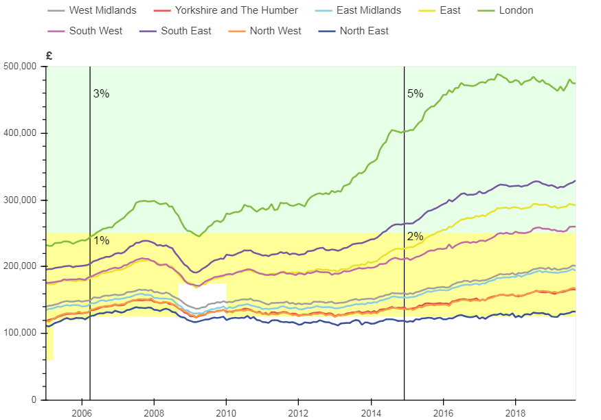
Image .csv .xlsFigure 11 shows the average house price for all regions in England alongside shaded areas that represent the tax thresholds for Stamp Duty at a given point in time. For example, in March 2005, the first-tier base threshold increased from £60,000 to £120,000. The second-tier threshold remains steady at £250,000 throughout the period.
Plotting the average house price against these thresholds is useful to demonstrate the impact that changes in house prices have on the Stamp Duty Index. Consider that any property sold with a price within the unshaded area pays no Stamp Duty at all. When modest growth in average house price occurs above the lower threshold, it is likely to have a higher impact on the percentage rate of growth in Stamp Duty yield.
As a brief hypothetical example: if 1,000 properties sell for £126,001, then £1,000 of the value of those properties would be above the basic threshold of £125,001 and be subject to the 2% tax rate (the current rules), generating £20,000:
1000 × £1000 ×0.02=£20,000
If those same houses rise to £135,001 in the next period, then they would have experienced a 7.1% rise in prices from one period to the next:
But in the new period, the Stamp Duty yield would be £200,000, as £10,000 of each property’s value is now taxable at 2%:
1000 × £10,000 ×0.02=£200,000
This represents a rise of 900% in the Stamp Duty tax yield from the last period.
Average house prices in London have made significant inroads into the second tax tier of Stamp Duty over the 15-year period. Couple this with the tax rate changes occurring in December 2014 (in the first tier it doubles from 1% to 2% and in the second tier it jumps from 3% to 5%) and it is clear that London house prices are having a big impact on the overall Stamp Duty Index.
All other English regions except the North East have experienced growth, with average house prices for the South West, South East and the East of England all now residing within the second tax tier. Average house prices in the North East of England have been the most stable, only recently rising back into the first tax tier around 2018. When viewing a regional Stamp Duty Index for this region, we would expect to see little recovery from the introduction of the marginal tax rate.
The missing segment from the tier one shaded area displays the tax holiday that was introduced in September 2008 to stimulate the housing market following the economic downturn. The average house prices for several regions is below the basic threshold during this period, which could explain why the Stamp Duty Index suffered such a sharp decline over the same period.
Figure 11: Average house prices have risen significantly in the past 15 years, particularly in London
UK, Jan 2005 to Sept 2019
Source: Office for National Statistics - Consumer price inflation
Notes:
- The average house price data in Figure 11 is available as an interactive chart in section 5 of the UK House Price Index: September 2019.
- The shaded areas represent the change in the tax thresholds for Stamp Duty Land Tax in the period observed. White is where no tax is paid, yellow is the first tier and green is the second tier.
- The black vertical lines represent a change in the Stamp Duty tax rates for the tax tiers shown. The percentage rate applicable to each tier is annotated at the start of the period for which it is applicable. For example, a tax rate of 5% is applicable to the second tax tier from December 2014 to September 2019. For more information on tax rates and tiers please read the sections above.
Download this image Figure 11: Average house prices have risen significantly in the past 15 years, particularly in London
.png (77.1 kB) .xlsx (28.6 kB)
An experimental buyer status column has been available in the house prices dataset from January 2012. Coincidentally, this was the date in which the first period of first-time buyers’ relief (FTB), applicable between April 2010 and December 2011, was taken away, and so the effects from this period on the Stamp Duty Index are unobservable. For the current period of FTB, however, the effects are observable, and these are illustrated by Figure 12 and Figure 13 showing the indices and difference in growth respectively.
The introduction of FTB causes a sharp fall in the Stamp Duty Index over the December 2017 period, after which the index closely follows the growth rate of the index calculated without FTB. The difference in month-on-month growth between the index with FTB and without for the 12 months following the introduction of FTB is on average a 12.6% decline.
Although the column used to make this distinction makes a significant assumption about the nature of cash buyers (that they are former owner-occupiers) and hence is experimental, the difference displayed in Figure 13 is too significant to ignore. The Stamp Duty Index with the effect of FTB is used in the headline results and the impact of this new estimate for Stamp Duty is explored in the following section.
Figure 12: The introduction of first-time buyers’ relief in December 2017 caused a significant fall in the Stamp Duty Index
UK, Jan 2005 to Sept 2019
Source: Office for National Statistics - Consumer price inflation
Download this chart Figure 12: The introduction of first-time buyers’ relief in December 2017 caused a significant fall in the Stamp Duty Index
Image .csv .xls
Figure 13: The introduction of the first-time buyers’ relief in Dec 2017 caused on average a 12.6 percentage point reduction in the annual growth
UK, Jan 2015 to Sept 2019
Source: Office for National Statistics - Consumer price inflation
Download this chart Figure 13: The introduction of the first-time buyers’ relief in Dec 2017 caused on average a 12.6 percentage point reduction in the annual growth
Image .csv .xls5. What are the impacts of these changes?
OOH(NA)
The component weights of the owner occupiers’ housing costs using the net acquisitions approach (OOH(NA)) are derived from national accounts data that are open to revisions (Table 1). These revisions have been incorporated into the latest index and have impacted the growth of the index. Similarly, including the new Stamp Duty Index (including first-time buyers’ relief) in the calculation of the index has also had an impact as part of the component 0.1.1.3 “Other services related to acquisitions” (an aggregate of Stamp Duty and transfer costs).
These impacts are shown by Figure 14, which displays the year-on-year growth rate of OOH(NA) with and without the changes described in the previous paragraph, along with bars that show the difference in growth at each period. The amount of difference attributed to each change is distinguished by the fill colour of the bars, as described in the legend of the figure.
When considering the absolute values over the total observed period, the average impact of the new Stamp Duty methodology on the growth of OOH(NA) each period is 1 percentage point: this is the average of the impact when disregarding whether that impact is positive or negative. When considering the sign of the values, the average impact of the new Stamp Duty Index is 0.4 percentage points on the growth of OOH(NA) each period. In the period of economic downturn following the global financial crash and the subsequent recovery period, the impact can be as much as 4.2 percentage points.
The average absolute impact of the revised national accounts expenditures on the growth of OOH(NA) is 0.6 percentage points each period. When considering the impact of both positive and negative contributions over the period observed, the result is that the revised expenditures have had a negligible positive impact (0.02 percentage points) on average on the growth of OOH(NA) over the period.
Figure 14: 12-month growth rate of OOH(NA) with and without the new stamp duty methodology and revised expenditures
UK, Jan 2006 to Sept 2019
Source: Office for National Statistics - Consumer price inflation
Download this chart Figure 14: 12-month growth rate of OOH(NA) with and without the new stamp duty methodology and revised expenditures
Image .csv .xlsOOH(payments)
The use of the revised national accounts expenditure values in the derivation of component weights also impacts the owner occupiers’ housing costs using the payments approach through the Stamp Duty, and major repairs and maintenance components.
The impacts are shown in Figure 15, which displays the year-on-year growth rate of OOH(payments) with and without both changes as time series, overlain on bars that show the difference in growth at each period. The amount of difference attributed to each change is distinguished by the fill colour of the bars, as described in the legend of the figure.
When considering the absolute values over the total observed period, the average impact of the new Stamp Duty methodology on the growth of OOH(payments) each period is 1.3 percentage points. When considering the sign of the values, the overall impact of the new Stamp Duty Index is a positive impact on the growth of OOH(payments) in the period observed, of 0.6 percentage points.
The expenditure weight for the Stamp Duty component in OOH(payments) doubled in the period from 2010 to January 2017, from 8 to 16, reflecting an increase in national accounts expenditures for Stamp Duty. This means that smaller movements in the Stamp Duty Index will have a bigger impact on OOH(payments) in the later periods (from 2017) when compared with similar movements in the earlier periods (pre-2010).
The average impact (when considering absolute values) of the revised expenditures on OOH(payments) each period is 0.2 percentage points, although when considering the sign of the values, the result is a 0.1 percentage points positive impact on average each period.