1. Abstract
In this article we estimate the value of recreational and aesthetic services provided by green and blue spaces in urban areas in Great Britain that is capitalised into property prices.
To do so, we create a unique house-level dataset by linking data from a property website to a comprehensive data set of urban green spaces, as well as data on air and noise pollution, and measures of school distance and quality. We extend the traditional hedonic pricing approach by using machine learning techniques to flexibly model house prices.
Unlike standard hedonic pricing via linear regression, our model does not rely on any assumptions regarding the relationship between house prices and the wide range of structural, neighbourhood and environmental characteristics.
We compute partial dependency plots to display the marginal effects of green and blue spaces on house prices and test whether they are linear. We then compute estimates of the value of cultural (recreational and aesthetic) services provided by green and blue spaces in urban areas.
Nôl i'r tabl cynnwys2. Introduction
Almost one-third of the urban area in the UK consists of natural land and green or blue spaces . Urban green spaces1 are a type of natural asset that provide society with a range of benefits. The Office for National Statistics (ONS), together with the Department for Environment, Food and Rural Affairs (Defra), are developing natural capital accounts for the UK to offer a comprehensive and consistent framework to organise environmental information so that the benefits of nature are better recognised.
In this article we focus on estimating the value of the cultural services of urban green spaces. Cultural services of green spaces primarily consist of recreation and aesthetic views, which are difficult to value, because they can be enjoyed for free. Following the previous literature2 , we estimate the value of these cultural services using a hedonic pricing approach. The aim is to isolate the contribution of urban green and blue spaces to property prices, and account for the effect of other environmental services such as noise and air pollution reduction.
To do so, we create a unique house-level dataset by linking data from a property website to comprehensive information about availability of urban green and blue spaces. We also add data on air and noise pollution and measures of school distance and quality. As a measure of recreational service, we focus on the distance to the nearest green and blue spaces as well as the area of all green and blue spaces within 500 metres of the property. Based on the property description from the website, we assess whether the property has a view over a green or blue space and use this information as a measure of aesthetic services.
Our main contribution is to extend the traditional hedonic pricing approach by using a boosted tree method to flexibly model house prices. Unlike standard hedonic pricing regression, our model does not rely on any assumptions regarding the relationship between house prices and the wide range of structural, neighbourhood and environmental characteristics. As a result, we can test if distance from and area of green and blue spaces jointly affect property prices and if these effects are linear and differ across geographical areas.
Another advantage is that we can control for observed factors in a more flexible way, therefore reducing the bias caused by misspecification of observed variables. It also allows us to capture spatial correlation by using a flexible function of longitude and latitude.
We find that the average contribution of green and blue spaces to property prices is £2,813.8, which is about 1.2% of the average property price in our sample.
The remainder of this article is structured as follows. In the next section we describe the data we use in this article and report some summary statistics. We then present the methodology used to model property price and estimate the effect of green and blue spaces on property price. We then present our results, and finally discuss the next steps.
Notes for: Introduction
See Irwin, 2002 ; Nicholls and Crompton (2005), Gibbons and others 2014; Schläpfer and others 2015).
3. Data and summary statistics
Data
Zoopla
We use data on property transactions from Zoopla, a UK-based property website. The dataset was originally provided for the previous iteration of this project by Zoopla Limited to the Urban Big Data Centre (UBDC) and includes information for over 1 million properties sold in Great Britain between 2009 and 20161.
Information includes location, number of bedrooms, number of reception rooms, property type, for sale or rent, asking price, sale price and so on. The data provided by Zoopla also contain a description of the property, which we use to fill in missing information about property type and number of bedrooms. We also use the textual description to extract additional characteristics, for example, whether it has a garage, has been recently renovated, or has a fireplace.
Most importantly, we examine the textual description associated with each property to determine whether that property has a view over a green or a blue space, such as a park, a river or the sea. Unlike studies that use a geographic information system (GIS) to detect views over green spaces (for example, Lake and others, 2000; Paterson and Boyle, 2002) we use contextual-based detection in the description:
first we identify descriptions that mention the following key words: overlook, views, backing, surrounded, outlook, look, opposite
we then examine whether the 40 preceding or following characters contain a set of words indicating green or blue spaces2
It should be noted that this measure of a view is experimental. Validating the quality of this derived variable is challenging since we do not have any true information as to whether a property has a view or not. A small amount of manual work was carried out in order to check the results of the contextual matching – which seemed relatively accurate – but false positives and false negatives are still likely to exist.
Ordnance Survey
In the previous iteration of this project the Ordnance Survey (OS) created a wide range of variables that may influence residential property prices for the purposes of the hedonic pricing method (HPM).
These variables were derived through the geospatial analysis of multiple OS datasets, both open data and premium data available through the Public Sector Mapping Agreement (PSMA), as well as other third-party datasets, all government published data, from the Office for National Statistics, Land Registry, Natural England and Natural Resources Wales.
The variables produced by the OS have been re-used for this project. The main environmental variables are the distance to publicly accessible green spaces (PAGS) and blue space, as well as the area of PAGS, blue spaces and natural land cover within 100, 200 and 500 metres of the property3. The precise definition of natural land cover, PAGS and blue space is:
natural land cover – any land cover classified as being natural in type, for example, grassland, heath, scrub, orchards, coniferous trees and so on; it does not include inland water bodies and can range from large woodland areas to small grass verges
publicly accessible green spaces – Ordnance Survey defines the following as types of green space: public parks or gardens, play spaces, playing fields, sports facilities, golf courses, allotments or community growing spaces, and religious grounds and cemeteries; these spaces contain natural land cover and can also include some blue space, for example, a park that has a lake within it
blue space – all inland water bodies, for example, rivers, lakes, ponds, canals and so on
We also use OS OpenData to calculate: approximate minimum distance to a railway line and approximate minimum distance to the coast. The coast is approximated by the high water line at a reduced resolution of 1/80 to save computation time as the original file is extremely large. The motivation for creating this variable is to account for houses that potentially had little access to PAGS but were near the sea. We calculate the minimum distance by matching the coordinates of houses to the nearest coordinates of the coastline data.
OS data were provided as a combination of a bespoke dataset and other OS open data. The open data were used under the Open Government Licence.
School data
There is a strong correlation between house prices and proximity to school4 . We incorporate data on proximity to schools using data on school location and quality from Ofsted and Estyn, the respective English and Welsh school inspection bodies. We were unable to include data on Scottish schools as Education Scotland only inspect a sample of schools and educational establishments are not given an overall inspection outcome in the same way that Ofsted and Estyn provide. We link the school data to our sample of residential properties and compute:
distance to the nearest primary, secondary, and post-16 school
inspection rating of the nearest primary, secondary, and post 16-school
An important caveat is that that Ofsted is not responsible for the inspection of private schools in England, and as such, these educational establishments are not present in the data. However, private schools’ admission rules are typically not based on a catchment area and so may not affect our analysis too much.
School data from Estyn and Ofsted were used under the Open Government Licence.
Noise pollution
Noise pollution has been found to be associated to house prices (for example, Levkovich and others, 2016), and is likely to also be linked to green and blue spaces. Including data on noise pollution in our model helps us identify the cultural services of green spaces, as we hold noise and air pollution constant.
For the purposes of this project we have only focused on noise pollution data from major roads and major railways across England, Wales and Scotland produced by the Department for Environment, Food and Rural Affairs (Defra)5. This type of data exists in the form of a shapefile from which we can access spatial polygons with various assigned attributes including their boundaries and noise-class. The noise-class is defined over several bins:
- x ≤ 54.9 dB
- 55.0 ≤ x ≤ 59.9 dB
- 60.0 ≤ x ≤ 64.9 dB
- 65.0 ≤ x ≤ 69.9 dB
- 70.0 ≤ x ≤ 74.9 dB
- 75.0 dB ≤ x
There are several different measures of noise pollution that take the time of day into account. We chose the Lden measure, which indicates the 24-hour average noise level with separate weightings for evening and night periods. The noise levels are measured on a 10 metre grid at receptor height of 4 metres above the ground, and the polygons are then formed by merging the neighbouring cells with the noise classes described above.
The three different possible noise metrics as well as an explanation of what noise sources were included in the 2012 noise mapping dataset.
There is a more recent edition of the strategic mapping that was carried out in 2017. But as this lies outside the period which our Zoopla data covers, we decided to use the strategic mappings from 2012.
Noise pollution data from Defra were used under the Open Government Licence.
Air pollution
We also use air pollution data from Defra, which is produced every year under their Modelling of Ambient Air Quality (MAAQ) contract. For each pollutant a grid with a resolution of one square kilometre are produced for which the most recent modelling methodology (PDF, 12.4MB) was published in 2015 by Ricardo Energy and Environment.
All the measurement units of the pollutants used in this project are:
NO2: Annual Mean
CO: Annual Mean
SO2: Annual Mean
Ozone: DGT120 (number of days on which the daily max 8-hr concentration is greater than 120 µg m-3)
Benzene: Annual Mean
While the housing data span between 2009 and 2016, matching houses to an air pollution value from any single year for any pollutant was highly time-consuming. This meant that it was not feasible to match houses to the levels of air pollution that were present in the year that they were sold. Additionally, the levels of CO pollution were only available until 2010. So for consistency, only pollution data from 2010 are used.
Air pollution data from Defra were used under the Open Government Licence.
Defra air pollution datasets are available.
Index of Multiple Deprivation
We use the Index of Multiple Deprivation (IMD) (2015) in order to capture socio-economic characteristics across England and Wales at the Lower layer Super Output Area (LSOA) level. Including the IMD in our model allows us to account for various neighbourhood characteristics such as employment, education, health and crime. The IMD is included as LSOA rankings in our model. This offers more flexibility than using deciles.
Output Area Code
To further account for the socio-demographic characteristics of the local areas, we include the 2011 Output Area Classification (OAC) in our model. This geo-demographic classification is based on 2011 UK Census data and was derived by Gale and others (2016). The OAC aims to identify areas of the country with similar characteristics. Each output area (a cluster of postcodes, with an average of 125 households) is classified into one of 76 categories, which provide summary indicators of the social, economic, demographic and build characteristics of small areas.
National Grid UK
We also use publicly available data6 from © National Grid UK to derive several other variables such as the distance to the nearest substation, distance to the nearest tower and approximate distance to the nearest overhead line. These features could have a negative effect on house prices and are likely to be correlated with access to green spaces.
Sample restriction
We restrict our sample to properties in urban areas that were sold between 2009 and 2016 in England and Wales (because the school data were not available for Scotland). We remove duplicate records and the few records with missing values. We exclude the bottom and top 0.5% of the distribution of property price. Our analytical sample contains 1,101,012 observations.
Summary statistics
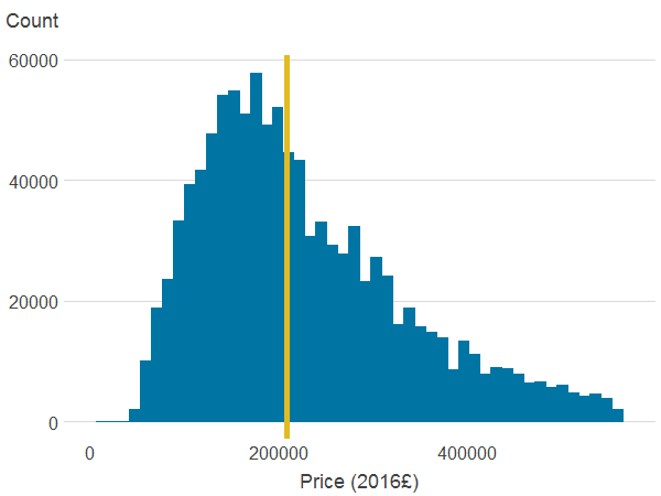
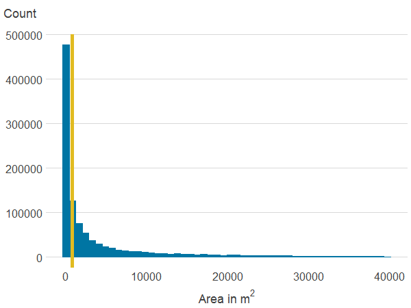
Table 4 in Appendix A shows summary statistics for our sample for the variables included in the model. In our sample the average price – where price is deflated and expressed in 2016 value – is £254,345. Figure 3 in Appendix A shows the distribution of the main variables and we can see that property prices follow a log-normal distribution, with a median of £208,007.
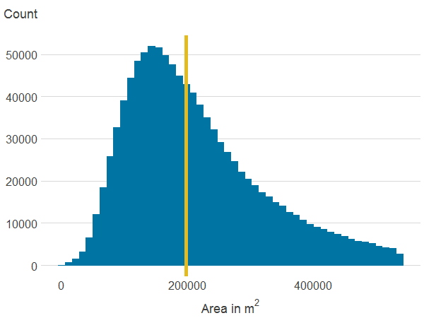
About 6.7% of properties in our sample have a view over green or a blue space. Residential properties in England and Wales are on average 257.2 metres away from a publicly accessible green space (PAGS) and 372.6 metres to a blue space. Within a 500 metres radius, the average area of PAGS is 159,736 square metres whilst the average area of blue space is 52,955 square metres. The average area of natural land cover is 236,710 square metres. However, as shown in Figure 3, which shows the distribution of the main variables, there is substantial variation in access to green and blue spaces.
In our sample, 25.7% of properties do not have any blue space site within a 500 metres radius and 6.4% have no access to any PAGS. By contrast, there is some natural land cover within 500 metres of all properties, and we can see from Figure 3 that natural land cover is more evenly distributed than PAGS or blue spaces.
Table 3 also shows summary statistics for all the covariates included in the model (except for Output Area Classification and geographical coordinates).
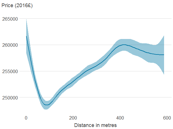
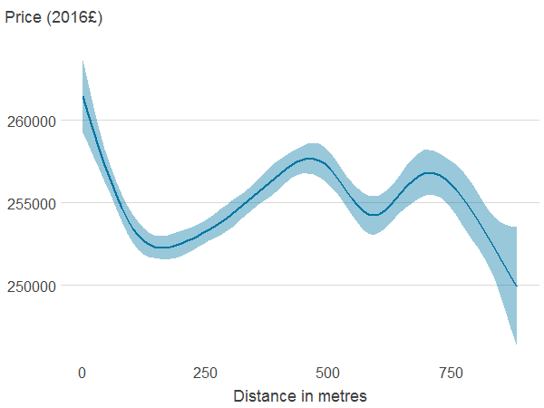
In Figure 4 in Appendix A we show how property prices vary with distance to an area of PAGS and blue spaces. The association between property price and distance to PAGS and blue spaces follows a U shape: prices are high for properties very close and relatively far from PAGS and blue spaces.
Properties far from PAGS and blue spaces may be more centrally located and therefore have access to other amenities or be more likely to be in expensive cities such as London. The association between property price, and area of PAGS and blue spaces is non-monotonic too, and difficult to interpret. This is because the area of PAGS and blue spaces are likely to be correlated with many other import factors that determine price. The area of natural cover is negatively associated with house prices, although price seems to increase with area at the top of the distribution.
Notes for: Data and summary statistics
In the previous iteration of this release, we used not only sold properties but also properties for sale or under offer. Further investigation of the data revealed that in many cases the same property was listed several times under different sale status. Therefore, we only focus on the records that are classified as sold.
List of words: green, woods, woodland, lake, river, riverfront, field, recreation, communal ground, reservoir, golf, quay, water, marina, sea, countryside, public, communal garden, reserve, forest, recreation, course, playing.
The area of PAGS within a given radius of the property includes the total area of the PAGS that have an access point within a given distance from the property.
See for instance this publication from Department for Education
The data are at: England Rail, England Road, Wales Rail and Wales Road, Scotland Rail and Scotland Road
Shapefiles for the transmission network can be found on the National Grid website.
4. Methods
The purpose of the article is to estimate the effect of urban green and blue spaces on property prices. Hedonic regressions are traditionally used to model the price of a property as a function of its attributes (Rosen 1974). Here we adopt a similar approach but use a non-parametric model to relax the assumptions associated with linear regression.
We model the property price as a function of environmental factors, house characteristics and neighbourhood and geographical characteristics:
where pricei,t is the real property price of house i sold at time t, deflated using the House Price Index (HPI). The vector of environmental characteristics envi is the main focus of our analysis and includes the distance to the nearest blue space, distance to the nearest publicly accessible green space (PAGS), area of all PAGS, blue spaces and natural land cover within 500 metres of the property1.
Our model also contains information on whether the property has a view over green or blue spaces. Whilst the distance and area of PAGS and blue spaces are measures of the recreational services provided by the natural environment, having a view over a green or a blue space can be seen as an aesthetic service.
hci,t is a vector of house characteristics. It includes number of bedrooms, property, building and garden area (square feet) and property type. We also derive a set of attributes from the description, such as period of the house (for example, Georgian, Victorian, Edwardian), and features that are likely to influence property prices (for example, garage, presence of original features, whether the property has been renovated recently).
ni is a vector of neighbourhood and geographical characteristics. It contains distance to amenities other than green and blue spaces such as transport infrastructures (for example, bus station, railway station), retail area and workplace centroid, as well as distance to features that might negatively impact house prices (such as overhead line and substation). It also includes distance to the nearest school, and the quality of the nearest school, as well as measures of air and noise pollution (a detailed description can be found in the data section). The socio-economic characteristics of the local area are captured by the Output Area Classification, a 76-category socio-demographic classification based on 2011 UK Census data, and the Index of Multiple Deprivation (see data section for more details). To capture unobserved area characteristics (spatial dependence), we include in our model an unspecified function of longitude and latitude. This approach is very similar to the generalised additive models (Hastie and Tibshirani, 1986) commonly used to capture spatial dependence (Geniaux and Napoléone, 2008). We also include the year when the property went on the market ( yeart ) to capture time effect.
Most hedonic pricing studies use linear regression to model property price and therefore assume that each feature has a linear effect on (log) house prices and that this effect does not depend on the other features2. This is a very strong assumption in our case, because property prices are likely to be a complex function of house characteristics, amenities and location: for instance, the effect of environmental amenities may be larger in parts of the country, or for properties with specific attributes. Interaction terms can be added in linear regression models to introduce more flexibility, but this may lead to a large number of predictors, making it difficult to estimate in practice.
Relaxing the assumption that the effect of each variable is linear3 and independent allows us to better capture the effect of environmental characteristics on house prices: for instance, a large area of green spaces may increase house prices more if the house is close to a green space and also has large blue spaces nearby. The effect of environmental characteristics on price may also differ depending on the house characteristics and neighbourhood factors.
This approach allows us to see if environmental amenities have heterogeneous effects on price. Finally, controlling for other factors in a more flexible way reduces the magnitude of unobserved heterogeneity4 and allows us to capture spatial correlation by using a flexible function of longitude and latitude.
We use a tree-based model to obtain the estimate:
Decision trees are a non-parametric machine learning algorithm, which can be applied to both classification and regression tasks. Unlike linear regression models, which are parametric, decision trees make no assumptions about the functional form of the data or the distribution of any model parameters.
While linear regression models the entire dataset as one function, decision trees split the space into homogenous subspaces, and then model the subspace with a simple function (usually the average). The main advantage of decision trees is their ability to handle data generated by complex non-linear and non-monotonic multivariate functions. Because a single tree is unlikely to produce a very accurate model, we use extreme gradient boosting to generate an ensemble of trees. The individual trees are built sequentially such that the next tree in the sequence attempts to minimise the errors made by the previous tree. For a more detailed explanation about decision trees for regression, see Appendix B.
Estimation procedure
Here we give details about the estimation procedure of our model where we use the R library XGBoost to estimate our model. XGBoost is unable to handle categorical variables and only accepts numerical input. Therefore, categorical variables should either be one-hot encoded or converted as numeric, as a tree-based model will split the numeric variable flexibly. However, this may be computationally more expensive.
All our categorical covariates excluding the Output Area Classification (OAC) are one-hot encoded. The OAC is converted as a numeric value to reduce the dimensionality of our dataset – 168 variables down to 93 variables.
We split the data into three partitions: train (56%), validate (30%), test (14%). The purposes of these three partitions are as follows:
train: the training partition is used to train the model in a supervised fashion; the model can access the true house prices for this partition of the data, which it uses to inform the learning process
test: we use the test set to tune the hyperparameters of our model to improve performance and generalisability
validate: this partition of the data is never shown to the model until we have decided on our final model; we use this dataset to conduct the analysis
The total size of the dataset (before partitioning) is approximately 1.10 million rows with 93 variables. Given that a model learns against 56% of these rows (roughly 600,000), training and testing is not a trivial task; due to the very large number of customisable hyperparameters that XGBoost gives the user access to, tuning is a lengthy process.
Grid search is the most thorough method for finding the optimal set of model hyperparameters. However, given the dimensionality of the problem (10 and over potential hyperparameters to tune ) this parameter space is far too large to search exhaustively.
In light of this we adopt a manual approach; focusing on tuning the most important hyperparameters: maximum tree depth, number of trees, learning rate, and optimise these as best as we can. Then we optimise the regularisation parameters: l1 & l2 regularisation, γ (minimum loss required to make a further tree partition on a leaf node), subsample of covariates to consider partitioning on per tree, level or node. The hyperparameters chosen for this analysis can be found in Appendix C in Table 6.
Once we have optimised our model against the test set, we calculate the appropriate performance metrics against the three partitions of the data. We have chosen to use the mean absolute error (MAE) for its ease of interpretability and the adjusted R squared ( Radj2 ). We prefer to report the Radj2 in this instance as we wish to penalise overcomplicated models with an excessive number of variables.
Interpreting the model
Our primary focus is to estimate the effect of environmental amenities on property prices. In a linear model, the coefficients show the conditional association between the independent variables and the dependent variable. In decision trees, assessing the relationship between independent and dependent variables is more complex. However, it is possible to compute marginal effects by estimating the partial dependency (PD) function, which shows how the prediction changes when the variables of interest vary (Zhao and Hastie, 2019).
We use PD plots to visualise the marginal effect of environmental amenities on house prices, conditional on all the other variables included in our model. We show the estimates of the marginal effect of PAGS and blue spaces separately. The partial dependency function for PAGS is defined as the predicted value of house prices for different values of distance and area of PAGS, holding other factors constant. It is given as:
Where pags is a vector containing the distance to the nearest PAGS and the area of PAGS within 500 metres of the property. xi is a vector containing all the characteristics of property i . wi is a set of weights aiming to make our sample representative of the stock of residential properties. The weights are derived using data from the Valuation Office Agency breaking down the number of properties by property types, number of bedrooms and region5. For a given level of PAGS distance and area, the value of the PD function is calculated as a weighted average of the predicted values for all the properties in the sample (n), with area and distance fixed at this given level6. To avoid overfitting, we estimate f ̂pags (pags) on a validation dataset that was not used to train and test the model. Because pags has two dimensions (distance and area), the result f ̂pags is a function of two variables therefore should be plotted with three dimensions.
The relationship estimated via the PD function can only be interpreted causally if the error term does not contain any factor that influences both property prices and the availability of environmental amenities (ignorability assumption). To make this assumption more likely to hold, we include a wide range of neighbourhood characteristics in our model (distance to amenities, school quality, air and noise pollution, socio-economic classification – see data section for more details).
Also, our models can flexibly capture non-linearities and interactions between the characteristics, reducing the risk that functional misspecification biases the estimates.
Finally, we include an unspecified function of latitude and longitude to capture spatial autocorrelation. However, as with any observational study we cannot test the ignorability assumption and therefore we cannot be fully certain that our estimates reflect a causal relationship.
Valuation of monetary stock
To obtain an estimate of the average effect of green and blue spaces on house price, we estimate the difference between the predicted price based on the real data and the predicted price if there were no green and blue spaces5 :
where wi is a set of weights aiming to make our sample representative of the stock of residential properties. The average value of green or blue space is calculated based on all the properties that are in our sample, including those that have no access to green and spaces. We can obtain an estimate of the value capitalised into property prices of the cultural services provided by green and blue spaces by multiplying this estimate to the number of residential properties in the UK. The recreational services are measured by the distance and area of blue and green spaces whilst the aesthetic services are captured by the view over green or blue spaces. We obtain 95% confidence intervals via bootstrapping7.
Notes for: Methods
A linear regression assumes that
Or another specified functional form.
Omitted interaction terms would end up in the residual εi,t
A comprehensive list of tuneable hyperparameters can be found on the XGBoost Parameters Documentation
The weights are derived for property types X number of bedrooms X region cells. For each cell j, the weight is equal to
where nj is the number of properties of cell j in our sample, and Nj is the number of properties of cell j in the VOA data. A weight greater than one is applied to properties under-represented in the Zoopla data whilst properties that are over-represented are given a weight lower than one.This is very similar to the method used to compute marginal effects for generalised linear models.
We set areas of green and blue spaces to 0 and distance to 500 metres, and view of green or blue spaces to zero.
5. Results
Partial dependency plots
The partial dependency function shows the predicted house prices for various distance and areas of publicly accessible green space (PAGS), holding all other characteristics constant. It describes the joint effect of distance and area of PAGS on property price.
In Figure 1 we report the effect of distance and area on property price as percentage difference compared with being further than 500 metres away from any PAGS (and therefore having no area of PAGS within 500 metres of the property)1. To better display the effects of distance and area on estimated average property price, we plot the data in two different ways.
Panel A of Figure 1 displays how property price varies with the distance to nearest PAGS for various areas of PAGS within 500 metres of the property, holding all other characteristics constant. Panel B shows how property price varies by area of PAGS, for several various distances to PAGS.
Overall, we can see that being further away from a PAGS reduces property prices, for any area of PAGS. Having large areas of PAGS within 500 metres of the property is associated with an increase in property price.
Being close to large areas of PAGS attracts the largest premium: a property close to a large PAGS is on average about 3.5% (£8,664.0) more expensive than a similar property far from any PAGS. Whilst the effect of area is almost linear, both plots also show that the relationship between property price and distance is non-linear; plot A showing increasingly flat lines and plot B showing decreasing amounts of space between lines.
For example, for any fixed area, being 400 metres instead of 500 metres away from a PAGS makes a negligible difference to the estimated average property price, whilst the difference between 100 metres and 200 metres is substantial. A property with 100,000 square metres of PAGS within 500 metres decreases in average predicted value by 1.0% (£2,421.2) if moving from being very close to 100 metres, while an equivalent property moving from 400 metres to 500 metres will only decrease in average predicted value by about 0.1% (£229.6).
Figure 1a: Partial dependency plot between area of publicly accessible green space (PAGS) within 500 metres and distance to nearest PAGS
Distance
Source: Office for National Statistics
Notes:
- Partial dependency functions based on XGBoost model. The effect of distance and area on property price are expressed as percentage difference compared with being further than 500 metres away from any publicly accessible green space.
Download this chart Figure 1a: Partial dependency plot between area of publicly accessible green space (PAGS) within 500 metres and distance to nearest PAGS
Image .csv .xls
Figure 1b: Partial dependency plot between area of publicly accessible green space (PAGS) within 500 metres and distance to nearest PAGS
Area
Source: Office for National Statistics
Notes:
- Partial dependency functions based on XGBoost model. The effect of distance and area on property price are expressed as percentage difference compared with being further than 500 metres away from any publicly accessible green space.
Download this chart Figure 1b: Partial dependency plot between area of publicly accessible green space (PAGS) within 500 metres and distance to nearest PAGS
Image .csv .xls
Figure 2a: Partial dependency plot between area of blue space within 500 metres and distance to nearest blue space
Distance
Source: Office for National Statistics
Notes:
- Partial dependency functions based on XGBoost model. The effect of distance and area on property price are expressed as percentage difference compared with being further than 500 metres away from any blue spaces.
Download this chart Figure 2a: Partial dependency plot between area of blue space within 500 metres and distance to nearest blue space
Image .csv .xls
Figure 2b: Partial dependency plot between area of blue space within 500 metres and distance to nearest blue space
Area
Source: Office for National Statistics
Notes:
- Partial dependency functions based on XGBoost model. The effect of distance and area on property price are expressed as percentage difference compared with being further than 500 metres away from any blue spaces.
Download this chart Figure 2b: Partial dependency plot between area of blue space within 500 metres and distance to nearest blue space
Image .csv .xlsFigure 2 shows the joint effect of distance and area of blue spaces on house prices. These plots are obtained using the same method as that used to obtain the partial dependency plot (PDP) for PAGS but show how price varies when distance and area of blue spaces change, holding everything else constant. Results are expressed as percentage difference compared with being further than 500 metres away from any blue spaces2.
Overall, we can see that the relationship between area and distance to blue spaces and house price follows a similar non-linear relationship to the one found for PAGS. Properties close to large blue spaces (30,000 square metres) are on average 3.4% (£8,397.7) more expensive than comparable properties with little access to blue spaces. However, the effects of proximity to blue spaces diminish faster than the effect of proximity to PAGS.
We also estimate the marginal effect of having a view over a green or a blue space. We do so by taking an average model prediction where all houses have been fixed to have a view over a green or a blue space and subtract it from an average model prediction where all houses have been fixed to not have a view over a green or a blue space. We find that having a view over a green or a blue space increases property price by £5,369.7 (2.0%) holding everything else constant.
The value of urban green and blue spaces
As explained in the Methods section, we estimate the difference between the predicted price based on the real data and the predicted price if there were no publicly accessible green spaces (PAGS) nor blue spaces to obtain an estimate of the average effect of PAGS and blue spaces on property price. To simulate the absence of PAGS and blue spaces, we set areas of PAGS and blue spaces to 0 and distance to 500 metres, and view of green or blue spaces to zero.
In Table 1, we display estimates of the value of cultural services capitalised into property prices by year. Based on 2016 data, the average value of PAGS and blue spaces embedded in property prices is £2,813.8 [95% confidence interval (CI): 2,401.5 to 3,089.0], which is 1.2% of the average property price in our sample. This average is calculated on a sample that includes properties that have no access to PAGS nor blue spaces, and therefore can be readily used to obtain an estimate of the overall value of cultural services of urban green and blue spaces that are capitalised into property prices.
To do this, we need to multiply this figure by the number of residential properties in 2016 (27.7 million) in the UK2. We obtain an estimate of £77.9 billion [95% CI: 66.6 to 85.6 billion] for the stock value of PAGS and blue spaces capitalised into property prices. The estimate is lower than the estimate published in the last version of this study, in which we used a linear model. This is probably because our tree-based model captures more heterogeneity and reduces the amount of bias. Out of this total, 12.1% (£9.43 billion) can be attributed to aesthetic services measured by having a view over a green or a blue space), whilst the remaining can be attributed to recreational services.
| Year | Average value (£) | 95% CI lower bound (£) | 95% CI upper bound (£) | Average value (% of average price) | Stock value (£billion) | Aesthetic value (£billion) | Recreational value (£billion) | N properties (billion) |
|---|---|---|---|---|---|---|---|---|
| 2009 | 2,519.3 | 2,260.1 | 3,132.9 | 1.05% | 66.84 | 11.24 | 55.59 | 26.5 |
| 2010 | 3,274.8 | 2,965.1 | 3,647.5 | 1.36% | 87.42 | 10.84 | 76.59 | 26.7 |
| 2011 | 3,295.8 | 3,070.2 | 3,806.8 | 1.33% | 88.51 | 9.68 | 78.83 | 26.9 |
| 2012 | 3,427.0 | 2,997.9 | 3,725.4 | 1.37% | 92.56 | 10.59 | 81.97 | 27.0 |
| 2013 | 3,313.5 | 3,004.4 | 3,731.5 | 1.30% | 89.96 | 11.27 | 78.70 | 27.2 |
| 2014 | 3,249.0 | 2,877.9 | 3,590.1 | 1.29% | 88.72 | 10.89 | 77.82 | 27.3 |
| 2015 | 2,814.0 | 2,484.9 | 3,145.4 | 1.21% | 77.38 | 9.66 | 67.72 | 27.5 |
| 2016 | 2,813.8 | 2,401.5 | 3,089.0 | 1.19% | 77.98 | 9.43 | 68.55 | 27.7 |
Download this table Table 1: Value of cultural services of PAGS and blue spaces capitalised into property prices by year
.xls .csvIn Table 2 we show the estimates of the average value of cultural services of urban green and blue spaces capitalised into property prices by travel to work area (TTWA). We report both the absolute value and the value relative to the average property price in the area.
These estimates show the average contribution of PAGS and blue spaces to property prices in each TTWA. We observe substantial variation across TTWA. The average value of cultural services of urban green and blue spaces capitalised into property prices as proportion of average property price is highest in Bath (3.7%) and is above 2% in Manchester, Liverpool, Cardiff, Newcastle, Oxford, York, Cheltenham and Canterbury. The contribution of green and blue spaces to property price is about 1%. The variation in the value of cultural services capitalised into property prices across TTWA could be because of difference in the availability of green and blue spaces, but also to differences in returns to living close to green and blue spaces.
| Travel-to-work area | Average value (£) | Average value (% of average price) | 95% CI lower bound (%) | 95% CI upper bound (%) | N validation set | Avg. Distance Blue Spaces | Avg. Distance PAGS |
|---|---|---|---|---|---|---|---|
| Bath | 12,307.5 | 3.71% | 2.30% | 3.70% | 1,118.0 | 421.2 | 203.5 |
| Newcastle | 4,550.4 | 2.55% | 2.24% | 3.19% | 4,866 | 527.2 | 202.3 |
| Manchester | 4,469.1 | 2.47% | 2.09% | 2.73% | 14,161 | 282.2 | 219.4 |
| Liverpool | 3,999.1 | 2.46% | 1.91% | 2.57% | 5,702 | 430.4 | 223.2 |
| Cheltenham | 5,884.0 | 2.32% | 1.55% | 2.37% | 1,608.0 | 302.7 | 252.9 |
| Oxford | 7,758.0 | 2.25% | 1.64% | 2.81% | 2,281.0 | 298.3 | 284.9 |
| Cardiff | 4,213.5 | 2.07% | 1.38% | 2.22% | 4,916 | 289.8 | 258.5 |
| Canterbury | 5,606.2 | 2.04% | 1.69% | 2.33% | 1,478.0 | 274.1 | 302.4 |
| York | 4,330.3 | 2.03% | 1.39% | 2.22% | 1,857.0 | 337.0 | 244.3 |
| Chester | 3,602.3 | 1.95% | 1.58% | 2.34% | 1,438.0 | 323.8 | 280.8 |
| Cambridge | 6,030.2 | 1.92% | 1.21% | 1.88% | 2,986 | 320.6 | 243.6 |
| Leamington Spa | 5,004.9 | 1.90% | 1.57% | 2.42% | 1,375.0 | 308.9 | 282.1 |
| Leeds | 3,714.4 | 1.88% | 1.49% | 2.12% | 7,401 | 428.1 | 242.8 |
| Margate and Ramsgate | 4,173.1 | 1.87% | 1.20% | 2.12% | 1,138.0 | 462.5 | 213.2 |
| Slough and Heathrow | 7,097.1 | 1.77% | 1.52% | 2.13% | 8,497 | 316.2 | 238.0 |
| Poole | 5,384.8 | 1.76% | 1.29% | 1.90% | 1,568.0 | 368.0 | 264.1 |
| Exeter | 4,478.6 | 1.76% | 1.39% | 2.14% | 2,730.0 | 278.6 | 279.3 |
| Warrington and Wigan | 2,584.1 | 1.72% | 1.52% | 2.13% | 4,175 | 273.7 | 268.2 |
| Eastbourne | 4,729.8 | 1.70% | 1.07% | 1.92% | 1,829.0 | 335.8 | 269.9 |
| Preston | 2,735.9 | 1.64% | 1.12% | 1.87% | 2,591.0 | 246.4 | 263.6 |
| Huddersfield | 2,665.0 | 1.56% | 1.06% | 1.73% | 2,413.0 | 314.0 | 198.4 |
| Bristol | 3,868.3 | 1.55% | 0.96% | 1.60% | 7,047 | 345.9 | 206.7 |
| Worcester and Kidderminster | 3,085.3 | 1.53% | 1.14% | 1.77% | 2,394.0 | 298.8 | 263.6 |
| Bradford | 2,423.9 | 1.51% | 1.06% | 1.79% | 2,558.0 | 368.9 | 218.3 |
| Chelmsford | 4,722.0 | 1.50% | 1.12% | 1.64% | 3,649 | 286.4 | 293.9 |
| Nottingham | 2,643.6 | 1.49% | 1.16% | 1.71% | 7,775 | 407.9 | 255.3 |
| Stoke-on-Trent | 2,230.9 | 1.48% | 1.02% | 1.74% | 2,150.0 | 358.7 | 269.1 |
| Colchester | 3,455.0 | 1.46% | 1.16% | 1.82% | 1,610.0 | 347.5 | 302.0 |
| Ipswich | 3,082.4 | 1.42% | 0.83% | 1.53% | 2,981 | 408.8 | 260.7 |
| Hastings | 3,186.0 | 1.41% | 0.73% | 1.78% | 1,093.0 | 274.8 | 257.6 |
| Lancaster and Morecambe | 2,226.9 | 1.40% | 0.93% | 1.93% | 1,081.0 | 229.2 | 219.4 |
| Torquay and Paignton | 2,932.9 | 1.37% | 1.03% | 1.90% | 1,512.0 | 400.6 | 272.3 |
| Hull | 1,927.5 | 1.35% | 0.73% | 1.49% | 2,832.0 | 370.0 | 289.6 |
| Blackburn | 1,859.7 | 1.31% | 0.99% | 1.80% | 2,005.0 | 229.3 | 214.0 |
| Guildford and Aldershot | 5,152.6 | 1.31% | 0.96% | 1.65% | 4,772 | 305.1 | 242.6 |
| Stevenage and Welwyn Garden City | 3,866.9 | 1.30% | 0.81% | 1.34% | 2,085.0 | 402.8 | 251.9 |
| Bournemouth | 4,008.4 | 1.30% | 1.18% | 1.81% | 2,620.0 | 398.2 | 271.6 |
| Bedford | 3,166.9 | 1.28% | 0.77% | 1.46% | 1,291.0 | 385.7 | 274.0 |
| Birmingham | 2,478.5 | 1.26% | 1.08% | 1.63% | 14,529 | 342.3 | 267.3 |
| Milton Keynes | 3,107.2 | 1.26% | 1.02% | 1.70% | 3,637 | 311.0 | 278.0 |
| Southampton | 3,440.2 | 1.25% | 0.99% | 1.50% | 3,591 | 348.6 | 293.3 |
| Medway | 2,923.5 | 1.25% | 0.84% | 1.36% | 4,858 | 576.6 | 282.7 |
| Birkenhead | 2,147.5 | 1.23% | 0.85% | 1.49% | 1,978.0 | 428.3 | 226.7 |
| Derby | 2,164.4 | 1.23% | 0.89% | 1.37% | 2,918.0 | 397.2 | 255.2 |
| Blackpool | 1,912.8 | 1.22% | 0.74% | 1.64% | 1,241.0 | 475.9 | 256.8 |
| Middlesbrough and Stockton | 1,754.5 | 1.19% | 0.88% | 1.71% | 1,703.0 | 396.3 | 316.7 |
| Luton | 3,977.6 | 1.18% | 0.76% | 1.34% | 6,220 | 495.0 | 245.5 |
| Leicester | 2,205.9 | 1.16% | 0.94% | 1.39% | 5,576 | 308.7 | 282.5 |
| Sheffield | 1,943.7 | 1.15% | 1.06% | 1.62% | 6,372 | 422.8 | 246.6 |
| Brighton | 3,941.6 | 1.15% | 0.66% | 1.64% | 2,063.0 | 541.8 | 213.0 |
| Lincoln | 1,873.4 | 1.14% | 0.63% | 1.27% | 2,924.0 | 357.2 | 318.2 |
| Portsmouth | 2,714.4 | 1.12% | 1.08% | 1.56% | 4,482 | 350.5 | 281.8 |
| Chesterfield | 2,028.3 | 1.11% | 0.91% | 1.51% | 1,642.0 | 383.2 | 248.2 |
| Wakefield and Castleford | 1,736.1 | 1.09% | 0.84% | 1.55% | 2,289.0 | 419.5 | 237.6 |
| High Wycombe and Aylesbury | 3,720.0 | 1.05% | 0.66% | 1.09% | 3,377 | 396.3 | 293.1 |
| Chichester and Bognor Regis | 3,121.5 | 1.05% | 0.81% | 1.46% | 2,096.0 | 284.0 | 314.0 |
| Peterborough | 2,002.6 | 1.02% | 0.67% | 1.36% | 2,400.0 | 286.7 | 284.5 |
| London | 4,045.0 | 1.00% | 0.87% | 1.42% | 43,971 | 406.9 | 225.3 |
| Burton upon Trent | 1,687.5 | 0.99% | 0.45% | 1.17% | 1,230.0 | 330.6 | 282.0 |
| Swansea | 1,419.7 | 0.97% | -0.49% | 0.77% | 1,557.0 | 297.2 | 269.5 |
| Tunbridge Wells | 3,594.1 | 0.96% | 0.57% | 1.48% | 1,232.0 | 272.1 | 261.4 |
| Reading | 3,497.5 | 0.96% | 0.68% | 1.21% | 3,579 | 371.4 | 282.5 |
| Trowbridge | 2,025.9 | 0.90% | 0.43% | 1.13% | 1,815.0 | 289.2 | 302.0 |
| Gloucester | 1,863.1 | 0.88% | 0.18% | 1.00% | 1,403.0 | 302.0 | 247.1 |
| Telford | 1,413.5 | 0.79% | 0.49% | 1.24% | 1,291.0 | 350.4 | 315.0 |
| Worthing | 2,214.1 | 0.75% | 0.53% | 1.19% | 1,881.0 | 422.1 | 281.7 |
| Kettering and Wellingborough | 1,034.0 | 0.64% | 0.01% | 0.80% | 1,164.0 | 400.0 | 273.8 |
| Harrogate | 1,497.4 | 0.58% | 0.24% | 1.22% | 1,102.0 | 419.6 | 244.5 |
| Doncaster | 772.8 | 0.57% | 0.25% | 0.95% | 1,738.0 | 524.2 | 289.7 |
| Norwich | 1,255.2 | 0.57% | 0.48% | 1.08% | 4,351 | 411.7 | 291.4 |
| Wolverhampton and Walsall | 881.2 | 0.53% | 0.54% | 1.12% | 3,763 | 365.0 | 286.3 |
| Weston-super-Mare | 1,055.3 | 0.50% | -0.51% | 0.62% | 1,203.0 | 238.8 | 332.8 |
| Plymouth | 862.3 | 0.43% | 0.21% | 0.83% | 3,953 | 377.1 | 295.1 |
| Basingstoke | 1,285.8 | 0.42% | 0.28% | 0.80% | 1,750.0 | 651.9 | 319.5 |
| Mansfield | 486.4 | 0.35% | -0.13% | 0.71% | 2,225.0 | 596.3 | 248.8 |
| Northampton | 546.1 | 0.29% | 0.33% | 1.19% | 2,264.0 | 414.2 | 261.5 |
| Barnsley | 340.1 | 0.24% | -0.14% | 0.58% | 1,600.0 | 557.7 | 214.2 |
| Lowestoft | -192.0 | -0.10% | -0.64% | 0.45% | 1,064.0 | 254.1 | 289.3 |
| Swindon | -556.8 | -0.27% | -0.64% | 0.37% | 2,299.0 | 266.6 | 287.1 |
| Newport | -636.4 | -0.38% | -1.35% | 0.02% | 1,009.0 | 261.6 | 281.0 |
| Bridgend | -1,172.9 | -0.73% | -0.97% | 0.12% | 1,014.0 | 279.2 | 276.9 |
Download this table Table 2: Average value of cultural services of PAGS and blue spaces capitalised into property prices by travel-to-work areas (TTWA)
.xls .csvNotes for: Results
The reference price is £245,763.7.
6. Conclusion
In this article we estimate the value of recreational and aesthetic services provided by green and blue spaces in urban areas in Great Britain that is capitalised into property prices. We extend the traditional hedonic pricing approach by using machine learning techniques to flexibly model house prices.
The main benefit of using a non-parametric approach is that we make no assumptions regarding the relationship between house prices and the wide range of structural, neighbourhood and environmental characteristics. The gradient-boosted regression tree model we use allows us to control for observed factors in a fully flexible way, therefore reducing the bias caused by misspecification of observed variables.
We find that the distance to publicly accessible green spaces and blue spaces has a non-linear effect on house prices. We also find that the effect of the distance to PAGS and blue spaces depends on the area of the PAGS and blue spaces. For instance, a property close to a large PAGS is on average about 3.5% (£8,664.0) more expensive than a similar property far from any PAGS. Having a view over a green or a blue space further increases property price by £5,369.7 (2.0%).
We then used the results from this model to estimate the total value of PAGS and blue spaces that is capitalised into property prices. We find that PAGS and blue spaces increase property price by 1.2% (£2,813.8). We estimate that the total value of PAGS and blue spaces that is capitalised into property prices amounts to £77.9 billion.
An important limitation of this study is that we do not distinguish between the different types of PAGS, such as parks, playing fields, or allotments when modelling property price. Further work should look to model their respective effects on property prices as is it unlikely that they all equally valued by home buyers. This would allow for a more in-depth analysis into the value of each individual type of green space but would also improve the estimate for the overall value of PAGS.
Nôl i'r tabl cynnwys8. References
Gale, C. G., Singleton, A. D., Bates, A. G., and Longley, P. A. (2016). Creating the 2011 area classification for output areas (2011 OAC). Journal of Spatial Information Science, 12(2016), pages 1 to 27
Genius, G. and Napoléon, C. (2008). ‘Semi-parametric tools for spatial hedonic models: an introduction to mixed geographically weighted regression and goodtime models’ in Hedonic Methods in Housing Markets Springer, pages 101 to 127
Gibbons, S., Moura to, S., and Rezende, G. M. (2014). The Amenity Value of English Nature: A Hedonic Price Approach. Environmental and Resource Economics
Hastie, T. J. and Trispirane, R. J. (1986). Generalized Additive Models. Statistical Science volume 1, pages 297 to 318
Irwin, E. G (2002) The Effects of Open Space on Residential Property Values. Land Economics Volume 78, pages 465 to 480
Lake, I. R., Lovett, A. A., Bateman, I. J. and Day, B., (2000). Using GIS and large-scale digital data to implement hedonic pricing studies. International journal of geographical information science volume 14(6), pages 521 to 541
Levkovich, O., Rouwendal, J., and Marwijk, R. Van. (2016). The effects of highway development on housing prices. Transportation, volume 43(2), pages 379 to 405
Nicholls, S. and Crompton, J. L. (2005), The impact of greenways on property values: Evidence from Austin, Texas, Journal of Leisure Research, volume 37, number 3, page 321
Paterson, R. W. and Boyle, K. J. (2002), Out of sight, out of mind? Using GIS to incorporate visibility in hedonic property value models, Land Economics, volume 78, number 3, pages 417 to 425
Rosen, S. (1974) Hedonic prices and implicit markets: Product differentiation in pure competition. J. Polit. Econ. volume 82(1), pages 34 to 55 (1974)
Schläpfer, F., Waltert, F., Segura, L. and Kienast, F. (2015) Valuation of landscape amenities: A hedonic pricing analysis of housing rents in urban, suburban and periurban Switzerland. Landscape Urban Plan volume 141, pages 24 to 40
Zhao, Q., and Hastie, T. (2019), Causal Interpretations of Black-Box Models. Journal of Business & Economic Statistics, 0(0), pages 1 to 10
Nôl i'r tabl cynnwys9. Appendix A: Summary statistics
| Characteristic Vector | Component Variables | Sources |
|---|---|---|
| Structural | Number of bedrooms | Zoopla |
| Property area (square feet) | ||
| Property type, such as house, bungalow, flat | ||
| Property attributes based on description (for example, garage, double glazing) | ||
| Property area (square feet) | Ordnance Survey | |
| Neighbourhood | Distance to railway station | Ordnance Survey |
| Distance to local labour market | ||
| Distance to nearest transport infrastructure | ||
| Distance to nearest retail cluster | ||
| Distance to nearest schools | OFSTED; ESTYN | |
| Rating of nearest school | ||
| Socio-economic | IMD, OAC | ONS |
| Environmental amenities | Distance to green space | Ordnance Survey |
| Distance to blue space | ||
| Area of Natural Features in 500 metres radius of property (square metre) | ||
| Area of functional green space in 500 metres radius of property (square metres) | ||
| Area of blue space in 500 metres radius of property (square metre) | ||
| Function of green space | ||
| Area of residential garden (square metre) | ||
| Distance to railway line | ||
| View over green or blue space | Zoopla | |
| Air pollution | DEFRA | |
| Noise pollution | ||
| Distance to coast | ||
| Distance to substation, tower, overhead lines | UK National Grid |
Download this table Table 3: Variables included in the model
.xls .csv
| Mean | SD | Min | Max | |
|---|---|---|---|---|
| Price | 254,345 | 168,312 | 49810.8 | 1,438,798 |
| Area of pagssfr within 100m | 21,104 | 147,256 | 0 | 12,382,576 |
| Area of blue space within 100m | 9,660 | 322,417 | 0 | 15,022,962 |
| Area of natural land cover within 100m | 16,363 | 28,093 | 0 | 1,020,796 |
| Area of PAGS within 200m | 48,793 | 216,844 | 0 | 12,562,617 |
| Area of blue space within 200m | 19,007 | 448,059 | 0 | 15,036,901 |
| Area of natural land cover within 200m | 49,522 | 51,960 | 0 | 1,349,563 |
| Area of pagssfr within 500m | 159,736 | 374,606 | 0 | 12,896,375 |
| Area of blue space within 500m | 52,955 | 727,502 | 0 | 15,150,068 |
| Area of natural land cover within 500m | 236,710 | 152,501 | 2080 | 2,042,351 |
| Distance to nearest transport infrastructure node | 564.0 | 539.9 | 7 | 9,578 |
| Distance to nearest workplace zone centroid | 296.2 | 184.9 | 0 | 10,703 |
| Distance to nearest railway station | 1735.8 | 1346.9 | 2 | 14,456 |
| Distance to nearest retail cluster | 358.7 | 316.9 | 0 | 6,978 |
| Distance to bua exterior ring | 1435.3 | 2374.4 | 0 | 17,542 |
| Distance to nearest pagssfr | 257.2 | 174.5 | 0 | 4,146 |
| Distance to nearest bluespace site | 372.6 | 272.6 | 0 | 3,631 |
| Num bedrooms (capped to 6) | 2.79 | 0.88 | 1 | 6 |
| Building area | 98.4 | 256.7 | 2 | 41543 |
| Residential garden area | 223.5 | 314.3 | 0 | 21039 |
| Single or multiple occupancy Multiple Occupancy | 0.14 | 0.347 | 0 | 1 |
| Single or multiple occupancy Single Occupancy | 0.86 | 0.347 | 0 | 1 |
| Period | 0.049 | 0.217 | 0 | 1 |
| Regency | 0.001 | 0.037 | 0 | 1 |
| Victorian | 0.04 | 0.196 | 0 | 1 |
| Georgian | 0.011 | 0.105 | 0 | 1 |
| Edwardian | 0.006 | 0.078 | 0 | 1 |
| Stove | 0.043 | 0.203 | 0 | 1 |
| Character | 0.035 | 0.185 | 0 | 1 |
| Renovated | 0.047 | 0.211 | 0 | 1 |
| Garage | 0.432 | 0.495 | 0 | 1 |
| View | 0.067 | 0.25 | 0 | 1 |
| Double glazing | 0.715 | 0.451 | 0 | 1 |
| Balcony | 0.038 | 0.191 | 0 | 1 |
| Cul de sac | 0.121 | 0.326 | 0 | 1 |
| Loft conversion | 0.009 | 0.094 | 0 | 1 |
| Basement | 0.009 | 0.093 | 0 | 1 |
| Fireplace | 0.246 | 0.43 | 0 | 1 |
| En suite | 0.155 | 0.361 | 0 | 1 |
| Decking | 0.108 | 0.311 | 0 | 1 |
| Open plan area | 0.118 | 0.322 | 0 | 1 |
| Nice rock worktop | 0.02 | 0.14 | 0 | 1 |
| Property type Bungalow | 0.026 | 0.16 | 0 | 1 |
| Property type Cottage | 0.006 | 0.077 | 0 | 1 |
| Property type Detached bungalow | 0.031 | 0.173 | 0 | 1 |
| Property type Detached house | 0.151 | 0.358 | 0 | 1 |
| Property type End terrace house | 0.062 | 0.241 | 0 | 1 |
| Property type Flat | 0.125 | 0.33 | 0 | 1 |
| Property type House - unknown type | 0.013 | 0.115 | 0 | 1 |
| Property type Link-detached house | 0.005 | 0.069 | 0 | 1 |
| Property type Maisonette | 0.011 | 0.107 | 0 | 1 |
| Property type Mews house | 0.002 | 0.05 | 0 | 1 |
| Property type Semi-detached bungalow | 0.021 | 0.145 | 0 | 1 |
| Property type Semi-detached house | 0.293 | 0.455 | 0 | 1 |
| Property type Studio | 0 | 0.015 | 0 | 1 |
| Property type Terraced bungalow | 0.001 | 0.036 | 0 | 1 |
| Property type Terraced house | 0.231 | 0.421 | 0 | 1 |
| Property type Town house | 0.02 | 0.14 | 0 | 1 |
| Near primary school rating Adequate | 0.117 | 0.322 | 0 | 1 |
| Near primary school rating Excellent | 0.191 | 0.393 | 0 | 1 |
| Near primary school rating Good | 0.666 | 0.472 | 0 | 1 |
| Near primary school rating Unsatisfactory | 0.026 | 0.158 | 0 | 1 |
| Primary dist to school | 3903.9 | 20343.4 | 0 | 326,326 |
| Near secondary school rating Adequate | 0.193 | 0.395 | 0 | 1 |
| Near secondary school rating Excellent | 0.217 | 0.412 | 0 | 1 |
| Near secondary school rating Good | 0.529 | 0.499 | 0 | 1 |
| Near secondary school rating Unsatisfactory | 0.061 | 0.239 | 0 | 1 |
| Secondary dist to school | 4592.1 | 20776.7 | 0 | 327,520 |
| Near post16 school rating Adequate | 0.146 | 0.354 | 0 | 1 |
| Near post16 school rating Excellent | 0.301 | 0.459 | 0 | 1 |
| Near post16 school rating Good | 0.504 | 0.5 | 0 | 1 |
| Near post16 school rating Unsatisfactory | 0.049 | 0.217 | 0 | 1 |
| Post16 dist to school | 5308.2 | 21830.8 | 0.1 | 329,425 |
| SO2 pollution | 2.345 | 1.553 | 0.3 | 31.2 |
| NO2 pollution | 20.84 | 6.532 | 1.6 | 62.2 |
| CO pollution | 0.221 | 0.01 | 0.2 | 0.28 |
| Benzene pollution | 0.534 | 0.126 | 0.1 | 1.84 |
| Ozone pollution | 1.493 | 0.91 | 0 | 8.84 |
| Noise road 0-54.9 | 0.738 | 0.44 | 0 | 1 |
| Noise road 55.0-59.9 | 0.095 | 0.294 | 0 | 1 |
| Noise road 60.0-64.9 | 0.045 | 0.206 | 0 | 1 |
| Noise road 65.0-69.9 | 0.024 | 0.152 | 0 | 1 |
| Noise road 70.0-74.9 | 0.012 | 0.108 | 0 | 1 |
| Noise road 75+ | 0.087 | 0.281 | 0 | 1 |
| Noise rail 0-54.9 | 0.981 | 0.138 | 0 | 1 |
| Noise rail 55.0-59.9 | 0.01 | 0.097 | 0 | 1 |
| Noise rail 60.0-64.9 | 0.006 | 0.075 | 0 | 1 |
| Noise rail 65.0-69.9 | 0.003 | 0.054 | 0 | 1 |
| Noise rail 70.0-74.9 | 0.001 | 0.03 | 0 | 1 |
| Noise rail 75+ | 0 | 0.016 | 0 | 1 |
| IMD rank E | 17782.8 | 9219.7 | 2 | 31,458 |
| IMD rank W | 1787.1 | 186 | 1 | 1,817 |
| Min dist to OHL | 9355.4 | 20455.4 | 8.2 | 336,367 |
| Min dist to tower | 9355.6 | 20455.4 | 8.2 | 336,367 |
| Min dist to substation | 12445.1 | 23807.7 | 25.8 | 403,572 |
| Approx dist to coastline | 21317.5 | 22230.4 | 5.5 | 90,003 |
| Approx dist to railway line | 1060.9 | 971.4 | 5.9 | 9,811 |
| N= 1,101,012 |
Download this table Table 4: Summary statistics
.xls .csv
Figure 3a: Property price
Source: Office for National Statistics
Notes:
- The line is the median.
Download this image Figure 3a: Property price
.png (4.5 kB) .xlsx (18.8 kB)
Figure 3b: Distance to nearest publicly accessible green space

Source: Office for National Statistics
Notes:
- The line is the median.
Download this image Figure 3b: Distance to nearest publicly accessible green space
.png (4.5 kB) .xlsx (18.5 kB)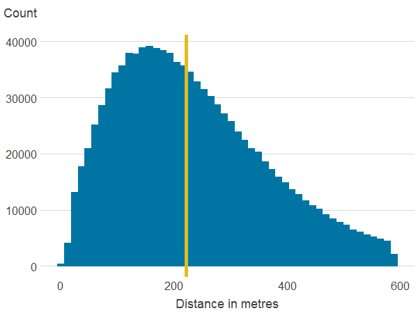
Figure 3c: Distance to nearest blue space

Source: Office for National Statistics
Notes:
- The line is the median.
Download this image Figure 3c: Distance to nearest blue space
.png (4.8 kB) .xlsx (17.8 kB)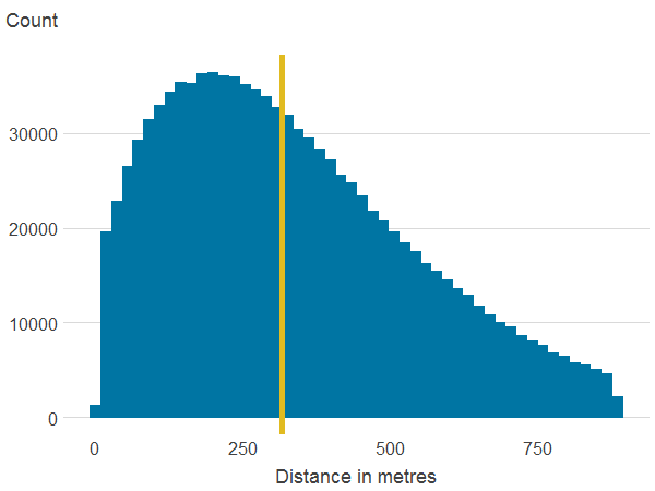
Figure 3d: Area of all publicly accessible green spaces within 500 metres

Source: Office for National Statistics
Notes:
- The line is the median.
Download this image Figure 3d: Area of all publicly accessible green spaces within 500 metres
.png (3.5 kB) .xlsx (18.6 kB)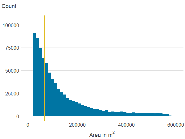
Figure 3e: Area of all blue spaces within 500 metres
Source: Office for National Statistics
Notes:
- The line is the median.
Download this image Figure 3e: Area of all blue spaces within 500 metres
.png (3.3 kB) .xlsx (18.5 kB)
Figure 3f: Area of all natural land cover within 500m
Source: Office for National Statistics
Notes:
- The line is the median.
Download this image Figure 3f: Area of all natural land cover within 500m
.png (4.5 kB) .xlsx (18.6 kB)
Figure 4a: Distance to nearest publicly accessible green space
Source: Office for National Statistics
Notes:
- Association between property price and the different features was estimated using generalised additive models. The solid line shows the estimated average property price for a given value of the distance from or area of blue or green spaces. 95% confidence intervals are shown in shaded areas.
Download this image Figure 4a: Distance to nearest publicly accessible green space
.png (5.8 kB) .xlsx (21.0 kB)
Figure 4b: Distance to nearest blue space
Source: Office for National Statistics
Notes:
- Association between property price and the different features was estimated using generalised additive models. The solid line shows the estimated average property price for a given value of the distance from or area of blue or green spaces. 95% confidence intervals are shown in shaded areas.
Download this image Figure 4b: Distance to nearest blue space
.png (5.8 kB) .xlsx (21.1 kB)
Figure 4c: Area of all publicly accessible green spaces within 500 metres

Source: Office for National Statistics
Notes:
- Association between property price and the different features was estimated using generalised additive models. The solid line shows the estimated average property price for a given value of the distance from or area of blue or green spaces. 95% confidence intervals are shown in shaded areas.
Download this image Figure 4c: Area of all publicly accessible green spaces within 500 metres
.png (4.8 kB) .xlsx (21.2 kB)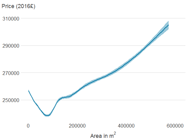
Figure 4d: Area of all blue spaces within 500 metres

Source: Office for National Statistics
Notes:
- Association between property price and the different features was estimated using generalised additive models. The solid line shows the estimated average property price for a given value of the distance from or area of blue or green spaces. 95% confidence intervals are shown in shaded areas.
Download this image Figure 4d: Area of all blue spaces within 500 metres
.png (5.7 kB) .xlsx (21.1 kB)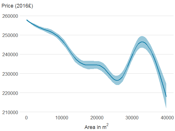
Figure 4e: Area of all natural land cover within 500 metres
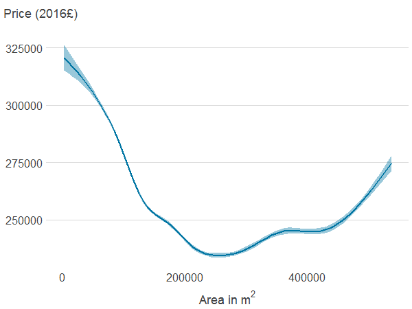
Source: Office for National Statistics
Notes:
- Association between property price and the different features was estimated using generalised additive models. The solid line shows the estimated average property price for a given value of the distance from or area of blue or green spaces. 95% confidence intervals are shown in shaded areas.
Download this image Figure 4e: Area of all natural land cover within 500 metres
.png (4.9 kB) .xlsx (21.2 kB)
10. Appendix B: Regression trees
Tree-based models for regression
Decision trees are a non-parametric machine learning algorithm, which can be applied to both classification and regression tasks. Unlike generalised linear models (GLMs) they are non-parametric and so make no assumptions about the functional form of the data or the distribution of any model parameters, which makes tree-based learners inherently different from GLMs.
Whilst the complexity of a GLM is only determined by the number of variables included in the model, the complexity of a decision tree has no upper limit and is likely to increase with more training data. The implications of this are that decision trees can be more computationally expensive to train, but are able to represent more intricate, non-linear relationships between variables, whereas a GLM (with no added interaction terms) assumes that all variables act independently of each other and have a linear relationship with the link function1.
Whilst GLMs model the entire dataset as one function, decision trees split the learning space into homogenous subspaces. Therefore, they can handle highly non-linear and non-monotonic multivariate functions.
The algorithm used to train a decision tree depends on whether the task is a regression or classification problem2. Since house price is continuous, this is a regression task.
A decision tree features three key elements: the root node, the internal nodes, and the leaf nodes. The root can be thought of as the base of the tree and contains the entire space of the data. If a decision tree consists of only a root, then regardless of the type of tree, all observations will be predicted to be the same value. This is equivalent to having a GLM with only an intercept term.
Leaving a decision tree in this state will almost never be enough for generating predictive power; complex problems involving large datasets – both in observations and dimensionality – will require the data to be split or partitioned according to some criterion. This criterion is dependent on the nature of the problem – classification or regression.
After the root has been initiated, the tree building algorithm will choose a way to partition the data such that the model minimises some function.
For regression, the data are partitioned in such a way that the algorithm tries to minimise the sum of the squared errors (SSE), given by:
Here, N is the total number of observations, yi is the true value of the quantity we are trying to predict, and y ̂i is the predicted value.
This process happens recursively until some stopping condition is met. Popular stopping conditions to prevent overfitting include imposing a maximum tree depth (the maximum number of levels that a tree can have) or a minimum leaf size (if a chosen split creates a leaf that contains less than this number then we do not perform the split).
Making predictions using classification or regression trees is relatively straightforward. For classification, each observation in the data will “belong” to a unique leaf dependent on the path along the tree that the observation followed. The final prediction will simply be the most common class occurrence at the leaf node. For the latter, the final prediction will be the average of all the true values at the leaf node.
Extreme gradient boosting with XGBoost
Before we outline a high-level overview of the theory behind of XGBoost, it is quickly worth noting that we briefly experimented with other tree-based regression models, including Random Forests. However, after some initial investigation we chose XGBoost as our primary modelling method as it consistently displayed better performance over the other algorithms.
For the purposes of this project we decided to use extreme gradient boosting as implemented by the XGBoost library in R. In the interest of conciseness, we have kept our explanation of XGBoost fairly high-level, however, the documentation created by the developers outlines the motivation and technical details in much greater depth.
As a general principle, gradient boosting is the process of using an ensemble of weak models to create an overall strong model. The term “ensemble” here simply means a collection of models, or in our case, a collection of decision trees. These individual trees are built sequentially such that the next tree in the sequence attempts to minimise the errors made by the previous tree. After enough boosting rounds we hope that the errors made by the most recent tree diminishes to the point where no improvement can be made while not overfitting to the data.
The XGBoost library provides a powerful implementation of gradient boosting for both linear and tree-based models. But as discussed earlier, we prefer not to make any assumptions about the functional form of the relationship between house prices and the variables, hence we choose tree-based models.
The library also gives us access to many hyperparameters that can be tuned to improve model performance including through regularisation techniques. This makes the modelling process more time-consuming, especially since individual models are not quick to train due to the size of the data. However, this is eventually rewarded with improved model performance compared with implementing less complex machine learning algorithms. The final model inference is presented in the Results section.
It is important to highlight that XGBoost models make predictions differently to the “classical” decision trees described in the previous section. As an XGBoost model is an ensemble of decision trees, each tree contributes to the overall final prediction, and for ensembles of trees the way in which each tree contributes depends on the algorithm.
For example, Random Forest and XGBoost models are both ensembles of decision trees but they make their predictions differently. In the case of XGBoost – as with a single decision tree – each observation in the data will belong to a unique leaf in the tree that has a weight w, and suppose we have N trees in our ensemble. Then the final prediction will simply be the sum of the weights across all N trees.
Notes for: Appendix B: Regression trees
GLM interaction terms can be added manually but this can very quickly increase the dimensionality of the data – something we prefer to avoid.
Here we present a high-level view of this process, but for more information please see classification and regression trees (PDF, 3.05MB).
11. Appendix C: Model hyperparameters
Here we present the values of the model hyperparameters. Any hyperparameters not listed here can be assumed to be their default values in version 0.81 of the XGBoost Python package.
| Hyperparameter | Description | Value |
|---|---|---|
| objective | Type of learning task to be carried out. | “reg:linear” |
| tree_method | Algorithm used for constructing trees. | “exact” |
| base_score | Initial model bias. | mean of house price in training data |
| max_depth | Maximum tree depth. | 16 |
| learning_rate | Shrinkage applied to tree weights. | 0.05 |
| n_estimators | Number of boosting rounds. | 400 |
| gamma | Minimum loss required to make a further partition in the tree. | 0 |
| subsample | Number of rows to randomly sample (without replacement when training a single tree). | 0.98 |
| reg_lambda | regularisation term on tree weights. | 2 |
| reg_alpha | regularisation term on tree weights. | 0.1 |
| col_samplebylevel | Subsample ratio of columns for a single tree | 0.6 |
| col_samplebylevel | Subsample ratio of columns for a single level | 0.6 |
| col_samplebylevel | Subsample ratio of columns for a single node | 0.6 |
| random_state | Random number seed – ensures reproducibility. | 123 |
Download this table Table 5: List of model hyperparameters
.xls .csv12. Appendix D: Model performance
| Partition | Mean Absolute Error (£) | Adjusted R2 |
|---|---|---|
| Train | 9579 | 0.9931 |
| Test | 29595 | 0.9087 |
| Validate | 29483 | 0.9091 |
Download this table Table 6: Performance metrics of the final model against all 3 partitions of the data
.xls .csvManylion cyswllt ar gyfer y Erthygl
vahe.nafilyan@ons.gov.uk, luke.lorenzi@ons.gov.uk
Ffôn: +44 (0)1633 455046