A simple guide to multi-factor productivity

Office for National Statistics (ONS) and other statistical offices publish regular estimates of “multi-factor productivity’” or MFP, but what exactly is MFP? This guide aims to give the non-expert user an understanding of MFP by explaining the underlying concepts through straightforward stylised scenarios.

But first, what is productivity and why does it matter? To understand productivity, it helps to think of the economy as a system that converts inputs into outputs, as shown in Figure 1.

Figure 1: Economic inputs and outputs

Download this image Figure 1: Economic inputs and outputs

.png (24.0 kB)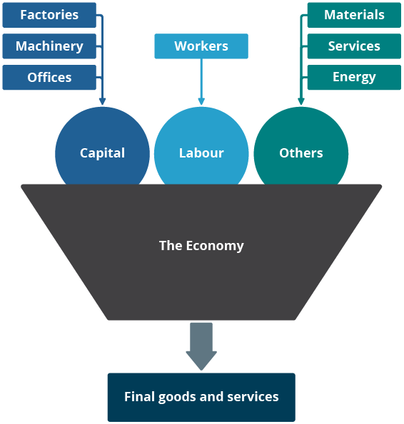

Outputs are the goods and services that we buy in shops and other outlets (and increasingly online). Economists refer to these as final goods and services, to recognise that when we buy, say, a chocolate bar, this requires non-final outputs such as cocoa, sugar and milk powder that are bought by the chocolate bar producer and transformed in the chocolate factory.

Economists usually classify inputs into three categories: labour, capital and other inputs. For the chocolate factory, labour input can be measured by the number of workers employed, although we prefer to measure the number of hours worked, which takes account of part-time and overtime working. Capital comprises the factory itself, the machinery within the factory and perhaps other items such as lorries to transport the finished produce, but also IT and communications equipment and so on. They might also include bought-in services such as security and cleaning, accountancy and legal services.

Productivity is simply the rate of conversion of inputs to outputs. The tricky part is measuring the inputs and outputs properly.

Productivity matters because most of us want to consume more goods and services over time. This bald statement may seem controversial – not all of us want to consume more chocolate bars for example. It would be more accurate to say that most of us want to enjoy higher living standards. Higher living standards may entail more consumption (where more can also mean better; for example, foreign holidays rather than domestic holidays), or enjoying more leisure time, that is, working fewer hours. It should be apparent that the only way in which most of us can enjoy higher living standards over time is by increasing productivity, that is, by increasing the rate of conversion of inputs to outputs.

A chocolate factory is a fairly complex organisation, with multiple inputs as set out previously and probably multiple different outputs (for example, chocolate bars of different sizes).

In the following example, “the economy” is represented by a small bakery, which produces “output” in the form of loaves of bread and sells its output to customers. For simplicity we assume that all loaves are of a standard size and quality. Our bakery uses inputs in the form of skilled and unskilled labour, capital including a baking oven and premises to operate in, and materials including flour, yeast and salt. On a day-to-day basis we assume that the bakery can vary its output of loaves only by varying the amount of labour and materials used. For example, the capacity of the oven might be limited to, say, 100 loaves per hour, and to keep things simple we might further assume that a skilled baker can operate at the same rate – thus mixing and preparing the dough for the next batch of 100 loaves while the previous batch is in the oven.

For the simplest measure of productivity, labour productivity, the only information we need is the number of loaves produced per time period (say, a day) and the number of hours worked.

Suppose the baker in our example works eight hours a day, and that the first hour each day is spent preparing the first batch of loaves for baking and the last hour for cleaning up, ordering materials and so on. This implies six-hourly baking cycles per day and if we assume that the baker works at full capacity, output of 600 loaves per day. Suppose also that our bakery employs a sales assistant to sell the output. The sales assistant might work for seven hours a day, as there would be no bread to sell in the first hour. (Note that while the baker might physically produce loaves of bread, the sales assistant provides the vital service of marketing them to customers.)

In this scenario, “output” would be 600 loaves per day, hours worked would be 15, so (daily) labour productivity would be 600 divided by 15 equals 40 loaves per hour (Table 1).

Taking this simple example as a starting point, how might productivity change? One possibility is that the baker and the sales assistant work fewer hours, say seven and six respectively each day. But if we maintain our assumption that two hours per day are needed for preparation and cleaning up, this would mean only five baking cycles, so output would be 500 loaves, hours worked would be 13 and labour productivity falls to 500 divided by 13 equals 38.5 loaves per hour.

Similarly, if the baker were to work less intensively, say only preparing 90 loaves per hour rather than 100, in the eight-hour day example (so 540 loaves a day), labour productivity would be 540 divided by 15 equals 36 loaves per hour.

Of course, if our baker was prepared to work more hours each day, he or she would be able to fit in more baking cycles and output would go up. But our baker might reasonably feel that eight hours per day is more than enough.

Suppose instead that our baker prefers to work seven hours per day but hires another baker to take over at the end of his or her shift. If the second baker also works 7 hours per day, at full capacity of 100 loaves per hour, then daily output will increase to 1,200 loaves (12 baking cycles, as two hours per day would still be required for preparation and clean up).

If we further assume that the bakery also hires a second sales assistant, so that sales can take place over 13 hours rather than seven hours, then total hours worked would be 27 and labour productivity would be 1,200 divided by 27 equals 44.4 loaves per hour, an increase on the starting position (Table 2).

An economist would say that this increase in labour productivity reflects increased efficiency in the use of labour and capital, for example, by reducing the proportion of down time relative to baking cycles.

In principle we could go further: hire yet another baker and run three shifts per day. For the purposes of this article we are going to preclude this option by assuming an absolute limit of 12 baking cycles per day.

Differences in the labour input from different types of workers are not accounted for when calculating labour productivity. The next section introduces quality-adjusted labour input, which breaks down labour input into hours worked and labour quality.

The first stage in moving from a simple measure of labour productivity to multi-factor productivity (MFP) is to take account of differences in labour input between different types of labour. At Office for National Statistics (ONS) we do this by making estimates of quality-adjusted labour input (QALI).

To calculate a measure of QALI we need some means of registering differences in types of labour input. Economic theory suggests that wages reflect the value that labour adds to production; for example, highly-paid footballers create more value than the ground staff.

A QALI measure accounts for these variations in labour composition or quality by weighting the hours worked of different “worker types” by their relative pay shares, that is, their shares of the total wage bill.

To illustrate this, we need to introduce hourly wages for our two types of workers. Let’s assume that the training and experience required of a baker is reflected in a going rate for bakers of £12 per hour, while the going rate for sales assistants is lower, at £8 per hour. Note also that QALI measures labour input between two periods or states of the world, so we will introduce QALI in relation to the difference between single- and double-shift working as in Tables 1 and 2.

This is shown in Table 3, in which the first three rows augment the figures in Table 1 with the relevant pay information, and the second three rows do the same for Table 2. The last three rows of the table combine information from both scenarios.

Looking in detail at the last three columns of Table 3, the column headed “Average pay shares (%)” calculates the simple average of the pay shares in the previous column across the two scenarios. This is not strictly necessary but is fairly standard practice in measuring MFP, and we will see other examples of the same approach later on.

The column headed “Change in hours” shows the change in hours for each type of worker and the total hours worked. However, the change is shown in log percentage points –that is, differences in natural logarithms – not arithmetic percentage points. This is calculated using the following formula:

Ln(14)-Ln(8) = 2.64-2.08 = 0.56 or 56%

Changes will be shown as log changes, as in this formula, for the rest of this article.

Log changes have the property that the change between two time periods (or, as here, two scenarios) is identical except for the sign whichever observation we use as the starting point. So, the log change in hours worked by skilled bakers from the double-shift scenario to the single-shift scenario would be negative 56%. (This is not the case for conventional percentage changes. The change from 8 to 14 is 75%, while the change from 14 to 8 is negative 43%).

Incidentally, it may be worth adding that while log changes can deviate from percentage changes, the differences between the two measures becomes small at the typical rates of change seen in economic statistics. So, a percentage change of, say, 2.0% would be 1.98% in log change terms.

The final column of Table 3 calculates the change in QALI. This is done is two steps. First, multiply the change in hours worked of each type of worker by their average pay share. Second, add these weighted changes together.

As can be seen, the result in this case is that QALI increases by 58.2% in moving from single- to double-shift working, compared with an increase of 58.8% in the total number of hours worked. This means that labour composition or "quality" has declined by 0.6%. This reflects a small reduction in the share of hours worked by the more skilled type of worker as captured in wage data; in this case, the baker.

How should we interpret this result? From a productivity perspective, the main point is that changes in labour quality are exactly comparable to changes in hours worked, so a change of, say, 1% in labour quality will have exactly the same effect on output as a 1% change in hours worked.

Recall from Tables 1 and 2 that labour productivity increased from 40.0 loaves per hour to 44.4 loaves per hour in moving from single- to double-shift working. Expressed as log changes, this is an increase of 10.5% (Ln(44.4)-Ln(40.0)).

Equivalently, we can calculate the change in output per hour as the (log) change in output (69.3%) minus the log change in hours worked (58.8%). This is calculated as follows:

69.3% − 58.8% = 10.5%

We now know that labour input adjusted for changes in labour composition grows slightly less than the growth in hours worked, so the growth in output per (adjusted) hour worked is calculated as:

69.3% − 58.2% = 11.1%

So, while overall labour input has increased, the rate of increase once we take account of changes in composition is slightly lower than the increase in the number of hours worked.

So far, we have focused entirely on labour inputs. The next stage is to take account of capital inputs to the production process. Capital input includes anything that provides an ongoing use to output without being used up in the production process. In our bakery, capital inputs would include things such as the oven and the building of the bakery; as they can be used in the production process more than once, they are not simply “used up” in each production cycle. Inputs such as the ingredients are not capital inputs, as once flour is used to make a loaf of bread, the same flour cannot be used again to produce another loaf of bread.

How do we measure capital inputs? For our published multi-factor productivity (MFP) estimates we estimate capital services. Conceptually, these are flows of productive services, directly comparable to flows of labour services measured by hours worked (and QALI). Measurement of capital services requires lots of information on the accumulation of capital assets over time, as well as a number of assumptions on the lives of different types of assets, how the productive efficiency of assets changes over their lifetimes, and the nature of the returns on capital. However, for our purposes, we can cut through this complexity by noting that this method essentially models the costs that firms would pay if they were to rent all their capital assets in competitive markets.

For our purposes, we will assume that our bakery rents its premises, oven and any other capital, and that the rents paid are fair reflections of the capital services provided by these assets.

Let’s assume that the bakery rents its premises for the equivalent of £75 per day. Assume further that the bakery rents an oven and associated equipment for the equivalent of £13 per day plus £10 for each hour that it is used (this is like leasing a photocopier and making payments based on the number of copies made). The different terms for the two types of capital reflect the fact that the life of premises is not materially affected by the intensity of its use, whereas equipment such as ovens will suffer wear and tear through use.

This information is summarised in Table 4, which follows the same format as Table 3. Note that unlike labour, we cannot distinguish a “quality” component for capital. As in Table 3, the column labelled “Average cost shares” shows the average share of each type of capital employed across the two scenarios. The change in capital services is then calculated as the change in costs of each type of capital weighted by its average cost share, and summed across both types.

Table 4 shows that a move from single- to double-shift working involves an increase of 34.0% in capital services employed in production. This may seem counter-intuitive: after all, the amount of physical capital employed has not changed. But in moving to double-shift working, the bakery is using its physical capital more intensively and therefore the flow of capital services has increased.

We should note that the example in Table 4 relies on rental charges fairly reflecting the value of each type of capital. In the real world, rental markets for capital assets are either thin or non-existent and most capital assets are owned directly by the firms that use them, albeit often financed by borrowings.

Moreover, even where rental markets exist, rental prices may include bundled labour services (such as a crane that is supplied with an operator) and margins for the rental organisation, and long-term rental terms will typically include an allowance for general inflation, which we are assuming away in our simplified scenarios.

Our multi-factor productivity (MFP) estimates measure output of goods and services in terms of gross value added (GVA). GVA is an estimate of the value of goods and services produced after deducting the cost of the intermediate inputs of goods and services consumed in the production process.

In our bakery, the costs of the intermediate inputs include the costs of materials such as flour, yeast, salt, electricity to heat the oven and so on.

In economic statistics, GVA for a particular firm or sector is exactly balanced by the costs of factor inputs, that is, the costs of labour and capital (plus a small tax component that flows to the government). This balance is brought about by assuming that any residual amount after accounting for labour and tax costs is a return to capital. Statisticians adopt this approach because in practice it is very difficult to measure returns to capital on a timely basis.

In our case, however, we have assumed a full set of information on labour and capital costs. Let’s assume that the costs of intermediate inputs are £0.50 per loaf. We will assume that the tax component is zero.

One option for our bakery would then be to set the selling price of its loaves to exactly match its costs (of intermediate inputs, labour and capital). But economists usually assume that small producers such as ours are price takers rather than price makers. So, let us instead assume our bakery sells its loaves at the going rate, which we will set at £1 per loaf.

What then, is the GVA of our bakery under the two scenarios set out and how is it divided between labour and capital? Table 5 provides more detail.

The first three columns of Table 3 describe the daily turnover of the bakery under the two scenarios. The cost of sales is the costs of intermediate inputs, which in our case are £0.50 per loaf. GVA is turnover minus cost of sales.

Does this presentation affect our measurement of output, which was specified earlier in terms of physical output of loaves of bread? The answer is that in a world in which prices and quality do not change, there is a direct relationship between physical output and the monetary value of turnover, shown in Table 5.

Notice also that in this example, growth of output measured by GVA is identical to the growth of turnover. This is because we have assumed a constant relationship between output of loaves and intermediate inputs, that is, we have assumed a fixed production technology.

In the last three columns of Table 5, labour and capital costs are copied from Tables 3 and 4, and the final column shows the residual profit, that is, GVA minus these costs. Other terms for residual profit are economic rent or supernormal profits and in economic theory, such profits are above and beyond those that are required to pay for the labour and capital used in production.

In the single-shift scenario, residual profits are zero, as GVA is exactly matched by payments to labour and capital. In the double-shift scenario, however, residual profits are strongly positive. In a later section we will explore how such profits might lead to an increase in production.

So far, we have separately measured the changes in quality-adjusted labour input and capital services between the two scenarios, and we have now established a measure of output growth in terms of gross value added (GVA).

The next step is to measure the respective weights of labour and capital in production. To do this we will use the cost information in Table 5, as shown in Table 6.

Note that, echoing our published multi-factor productivity (MFP) estimates, we again take the average labour cost share over the two scenarios. Note also that we define the capital cost share as one minus the labour cost share, that is, we are treating any residual profit as a return on capital.

In our simple example, labour costs account for 48% of GVA averaged over the two scenarios, with capital accounting for the remaining 52%. For comparison, the typical labour share in the UK economy is around two-thirds.

For any given change in output, multi-factor productivity (MFP) measures the amount that cannot be accounted for by changes in inputs of quality-adjusted labour and capital. Tables 3 and 4 show the changes in quality-adjusted labour and capital services respectively in our simplified example of moving from single- to double-shift working. Table 7 combines these changes with the change in output measured by gross value added (GVA) and the weighting information in Table 6.

The (log) change in quality-adjusted labour input (QALI) in Table 3 (58.2%) multiplied by the labour share in Table 6 (48.0%) gives a weighted contribution of 27.9% to the change in output.

Similarly, the (log) change in capital services in Table 4 (34.0%) multiplied by the capital share in Table 6 (52.0%) gives a weighted contribution of 17.7%.

The log change in output between our two scenarios is 69.3%. Subtracting the contributions due to changes in labour and capital inputs leaves a residual of 23.7% that cannot be attributed to changes in inputs and so represents a change in MFP. This is shown in Table 7.

As we saw earlier, if we divide output by hours worked we arrive at a simple measure of labour productivity. Table 8 shows how this can similarly be decomposed into three components:

• a component reflecting the change in capital services per hour worked, or capital deepening

• a component reflecting the change in labour composition

• a residual MFP component

Note that while capital services increase by 34.0% between the two scenarios, capital services per hour fall by 24.8% (the difference between these numbers is, of course, the growth in hours worked – 58.8%). So, the double-shift scenario is less capital intensive than the single-shift scenario.

The change in MFP (23.7%) is identical whether we decompose output growth or growth of output per hour. The fact that it is positive suggests that the single-shift scenario is inefficient: the bakery can become more efficient by using its fixed capital (that is, its premises and the fixed element of its baking equipment) more efficiently.

In the real world, changes in MFP can arise for a number of reasons including technological progress, economies of scale, changes in management techniques and business processes or more efficient use of factor inputs. MFP is linked, therefore, not to an increase in the quantity or quality of measured factor inputs but rather to how they are employed. In practice, MFP may also reflect measurement error of inputs and outputs. For example, if a firm employs new forms of capital that are not captured in our statistics, we would likely underestimate the growth of capital services and this could materialise as overestimation of MFP.

We saw in Table 5 that our bakery earns residual profits of £120 per day in the double-shift scenario. If we assume a cap of 12 on the number of hours that the bakery can operate per day, then this is the maximum profit that our bakery can generate, or alternatively, the optimal efficiency that our bakery can operate at, given the various assumptions that we have made. In terms of economic theory, our bakery is operating at the minimum point on its short-run cost curve.

But the existence of residual profits suggests that this is unlikely to be a sustainable position in the longer term. In economics, residual profits create incentives to expand production. This might take the form of new entry – rival bakeries opening in the neighbourhood and copying our bakery’s business model. Alternatively, the owner of our bakery may seek to expand their business by opening another bakery for themselves.

In either case, this is likely to compete down the residual profits available. Multiple competing bakeries may be forced to lower their prices to sell all their output and the additional demand for labour may put upward pressure on wages and the costs of intermediate inputs.

We leave exploration of the implications for productivity of such developments to a future article. In the meantime, we welcome comments on this article, which can be sent via email to productivity@ons.gov.uk.

The author acknowledges the contribution of Jessica Mohan, previously of Office for National Statistics.

• Productivity economic commentary: April to June 2018 draws together the main findings from official statistics and analysis of UK productivity to present a summary of recent developments (published 5 October 2018).

• Labour productivity, UK: April to June 2018 contains the latest estimates of labour productivity for the whole economy and a range of industries, together with estimates of unit labour costs (published 5 October 2018).

• Multi-factor productivity estimates: Experimental estimates to quarter 2 (April to June) 2018 presents quarterly estimates of multi-factor productivity (MFP), capital services and quality-adjusted labour input (QALI), including a range of industry breakdowns and analysis (published 5 October 2018).

• Quarterly UK public service productivity (Experimental Statistics): April to June 2018 contains the latest experimental estimates for quarterly UK total public service productivity, inputs and output (published 5 October 2018).

• Information and Communication Technology intensity and productivity contains new firm-level analysis to explore the relationship between the use of technologies and productivity (published 5 October 2018).

• Productivity development plan: 2018 to 2020 is a development plan that builds on recent improvements to our productivity statistics and looks at introducing new outputs, further improving our productivity statistics and consolidating our improvements to date (published 6 July 2018).

• How productive is your business is an interactive tool that helps businesses to calculate their productivity and compare their performance with other businesses in Great Britain (published 6 July 2018).