
1. Introduction
This supplementary material is intended to provide further detail on how the estimates in “the effects of taxes and benefits on household income (ETB)” are produced. It also provides further information and analysis on the measurement of inequality and examines the coherence of the ETB figures with other comparable sources.
Throughout this release, 2014/15 refers to the financial year ending 2015 and similarly for other years in this format.
Nôl i'r tabl cynnwys2. Redistribution of income
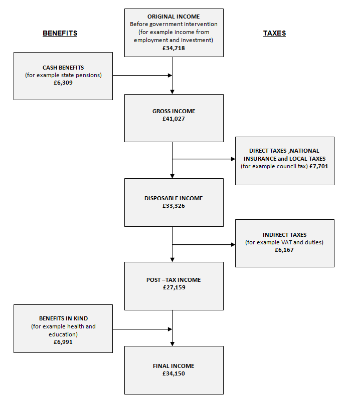
The five stages are:
- Household members begin with income from employment, private pensions, investments and other non-government sources. This is referred to as “original income”
- Households then receive income from cash benefits. The sum of cash benefits and original income is referred to as “gross income”.
- Households then pay direct taxes. Direct taxes, when subtracted from gross income is referred to as “disposable income”
- Indirect taxes are then paid via expenditure. Disposable income minus indirect taxes is referred to as “post-tax income”
- Households finally receive a benefit from services (benefits in kind). Benefits in kind plus post-tax income is referred to as “final income”.
Note that at no stage are deductions made for housing costs.
Diagram A: Stages in the redistribution of income
Source: Office for National Statistics
Download this image Diagram A: Stages in the redistribution of income
.PNG (21.7 kB) .doc (41.5 kB)
3. Original income
The starting point of the analysis is original income. This is the annualised income of all members of the household before the deduction of taxes or the addition of any state benefits. It includes income from employment, self-employment, investment income, private pensions and annuities which include all workplace pensions, individual personal pensions and annuities. This data is collected through the Living Costs and Food Survey (LCF; see background notes for further information on data sources). The term “annualised” refers to the estimate of income expressed at an annual rate based on the respondent's assessment of their “normal” wage or salary, subject to their current employment status. Where a respondent has been unemployed for less than one year, their normal wage or salary (for their last job) is abated for the number of weeks absence (where the respondent is off sick; receiving Employment and Support Allowance1; on a government training scheme; on maternity leave or receiving Jobseeker’s Allowance).
Similarly, for those in employment, this annualised estimate is “abated” for the number of weeks lost in the last 12 months due to sickness, maternity and so on. This is to avoid double counting wages and salaries and cash benefits. The abatement figure is taken as the number of weeks lost in the 12 months prior to interview.
About 98% of original income comes from earnings, private pensions (including annuities) and investment income. The very small amount remaining comes from a variety of sources: trade union benefits, income of children under 16, private scholarships, earnings as a mail order agent or baby-sitter, regular allowances from a non-spouse, allowances from an absent spouse and the imputed value of rent-free accommodation. Households living in rent-free dwellings are each assigned an imputed income (although this is counted as employment income if the tenancy depends on the job). This imputed income is estimated based on mortgage interest payment data for each of the regions and UK countries.
In addition to a wage or salary, some employees receive fringe benefits as part of their income such as company cars and rent-free accommodation. The company car benefit, together with the benefit from fuel for personal use, has been included in the analysis since 1990. Together these are by far the most important fringe benefit, accounting for around 60% of total taxable benefits by value according to the latest (August 2015) HM Revenue and Customs’ (HMRC) statistics.
The imputed income allocated to households is the taxable value of the benefit in accordance with HMRC rules. Since 2002, tax charges on company cars have been based on the car’s list price and official CO2 emission figure. The CO2 figure is converted to a percentage multiplier and applied to the list price for tax purposes. This determines the taxable benefit charge for the year. In 2012/13, the tax bands were amended to reflect falling average emissions for new cars in the UK. It should be noted that while the benefit is not taxable for those earning below £8,500, here the benefit has been allocated to all those with a company car regardless of the level of earnings or Income Tax band, as the benefit experienced by company car users is independent of these.
There was a change to the Company Car Fuel Benefit Charge in 2014. This affected employees with company cars who received free fuel from their employers and did not pay their employer back for the private use element of the fuel. This increased the multiplier used to calculate the cash equivalent of the benefit of free fuel provided to employees from £21,100 to £21,700. This change mainly affects the upper end of the income distribution.
Care should be taken in interpreting changes over time in the individual components of original income for each decile/quintile. Components such as self-employment income can be affected by both the amount earned by those who are self-employed, and the number of self-employed people with an equivalised disposable income2 in a given range in the sample, which can vary from year to year.
Notes for Original Income
Employment and Support Allowance (ESA) is a benefit for people who have a limited capability for work because of a health condition or disability. ESA was introduced in October 2008 and replaces Incapacity Benefit and Income Support paid on incapacity grounds.
See Disposable Income section for the definition of equivalised disposable income.
4. Gross income
The next stage of the analysis is to add cash benefits and tax credits to original income to obtain gross income. This is slightly different from the “gross normal weekly income” used in the LCF report “Family Spending”, as the gross income measure in “the effects of taxes and benefits on household income” analysis makes adjustments to abate for weeks of work lost for reasons discussed in the original income section.
Prior to 2013/14, cash benefits and tax credits were categorised as contributory or non-contributory. Contributory benefits, which include State Pension, widows’ benefits and Statutory Maternity Pay/Allowance, depend on the amount of National Insurance contributions that have been paid by, or on behalf of, the individual. Non-contributory benefits do not depend on National Insurance contributions. These include Income Support, Child Benefit, Housing Benefit, Statutory Sick Pay, Carer’s Allowance, Attendance Allowance, Disability Living Allowance, war pensions, Severe Disablement Allowance, Industrial Injury Disablement Benefits, Child Tax Credit and Working Tax Credit, Pension Credit, over 80 pension, Christmas bonus for pensioners, Government Training Scheme Allowances, student support, and Winter Fuel Payments. Some benefits/tax credits include both contributory and non-contributory elements, for example Jobseeker’s Allowance and Employment and Support Allowance (which is gradually replacing Incapacity Benefit and Income Support). From 2013/14, while it remained possible to identify the contributory and non-contributory elements of Jobseekers’ Allowance, this was no longer possible for Employment and Support Allowance, preventing the continued sub-division of benefits into these categories.
The roll out of Universal Credit began in 2013/14 in certain areas of greater Manchester and Cheshire, as well as Hammersmith and Inverness. From January 2015, Universal Credit became available to job seekers with children in 26 more areas across the country (with 6 job centre areas taking claims from families in November 2014).
When fully rolled out, Universal Credit will replace the following six means tested benefits and Tax Credits with a single integrated benefit for working age people:
- Income Support
- Income-based Jobseekers’ Allowance (JSA)
- Income-based Employment and Support Allowance (ESA)
- Housing Benefit
- Working Tax Credit
- Child Tax Credit
In the pilot areas, eligibility was limited to single jobseekers. The relatively limited scope of the pilot in 2013/14 meant that the impact of Universal Credit on the ETB data was negligible in that period. Since then, Universal Credit has been rolled out more widely, however, its impact impact remained limited on ETB data in 2014/15.
Figure A shows the extent to which cash benefits increase incomes, from the bottom fifth to the top fifth of households. It can also be seen that the majority of cash benefits go to the bottom two-fifths of households. In 2014/15, the average amount of cash benefits received by households was £6,300 per year, 15.4% of the average gross income (Reference Table 2). This proportion is broadly similar to 2013/14.
Figure A: Gross income by quintile groups of ALL households, financial year ending 2015
Source: Office for National Statistics
Download this chart Figure A: Gross income by quintile groups of ALL households, financial year ending 2015
Image .csv .xlsIn 2014/15 the average amount received from Employment and Support Allowance (ESA) increased by 86% compared with 2013/14. However, this increase should be seen in the context of a 53% fall in Incapacity Benefit and a 15% fall in Income Support, which ESA is gradually replacing.
Statutory Maternity Pay and Statutory Sick Pay is classified as a cash benefit even though it is paid through the employer.
Since 7 January 2013, where at least one spouse or partner in a household has income in excess of £50,000, a High Income Child Benefit charge has been applied. For incomes above £60,000 the High Income Child Benefit charge is equal to the amount of Child Benefit received. Those affected by the charge can either elect to stop getting Child Benefit (“opt out”) or pay any tax charge through self-assessment. There has been a decrease in the amounts received and the number of recipients of Child Benefit toward the upper end of the income distribution, with the top quintile receiving on average £35 (20%) less in 2014/15 than in the previous year. This suggests that many households who are subject to the High Income Child Benefit charge have elected to stop receiving Child Benefit, rather than pay any tax charge through self-assessment.
In line with national accounts, Child Tax Credit (CTC) and Working Tax Credit (WTC) have been reclassified and are now all recorded as cash benefits.
Income from short-term benefits (for example Jobseeker’s Allowance) is taken as the product of the last weekly payment and the number of weeks the benefit was received in the 12 months prior to interview. Income from long-term benefits (for example Disability Living Allowance) and from Housing Benefits is based on current rates.
In this analysis the State Pension is considered a cash benefit. As a result, for retired households (see Glossary in the Supporting information section), on average the State Pension accounted for 80% of the total cash benefits received (Reference Table 6). Reference Table 4 details the cash benefits that each non-retired quintile group received in 2014/15.
Most benefits, particularly Income Support, tax credits and Housing Benefit, are income related and so payments are concentrated in the two lowest quintile groups. However, the presence of some individuals with low incomes in high income households means that some payments are recorded further up the income distribution. Of the total amount of Income Support, tax credits and Housing Benefit paid to non-retired households, 47% goes to households in the bottom quintile group, an increase from 45% in 2013/14. As households at the lower end of the distribution tend to have more children (Reference Table 3), we also see higher levels of Child Benefit at this end of the distribution.
In 2014/15 cash benefits provided 45% of gross income for non-retired households in the bottom quintile group, while they account for just 2% of gross income in the top quintile. The payment of cash benefits therefore results in a significant reduction in income inequality.
Nôl i'r tabl cynnwys5. Disposable income
Income Tax, Council Tax and Northern Ireland rates and employees' and self-employed National Insurance contributions are grouped as direct taxes. When direct taxes are subtracted from gross income it forms disposable income. Taxes on capital, such as capital gains tax and inheritance tax, are not included in these deductions because there is no clear conceptual basis for doing so and the relevant data are not available from the LCF.
Figures for “Council Tax and Northern Ireland rates” include Council Tax (for households in Great Britain) and domestic rates (for households in Northern Ireland). Council Tax is shown after discounts, for example, the discount of 25% for single adult households. All Council Tax and Northern Ireland rates are shown after the deduction of Council Tax Support (formerly called Council Tax Benefit) and rate rebates. This is in line with the UK National Accounts which treat such rebates as revenue foregone. Up to and including 1995/96, these rebates were included as part of housing benefits.
Up to and including 2001/02, the figures for local taxes also included charges made by water authorities for water, environmental and sewerage services. From 2002/03, charges made by water authorities were treated as charges for a service rather than a tax, so the figures for Council Tax and Northern Ireland rates from 2002/03 onwards are not strictly comparable with those for local taxes up to and including 2001/02.
The tax estimates are based on the amount deducted from the last payment of employment income and pensions and on the amount paid in the last 12 months in respect of income from self-employment, interest, dividends and rent. The Income Tax payments recorded therefore take account of a household's tax allowances. Life assurance premium relief was deducted prior to 2011/12. However, from 2011/12 it was no longer possible to identify life assurance payments eligible for tax relief.
Households with higher incomes paid both higher amounts of direct tax and higher proportions of their income in direct tax. The top quintile group paid an average of £19,800 per household in direct taxes in 2014/15 (Reference Table 2). In contrast, the direct tax bill for households in the bottom quintile group was around £1,500 per year. These amounts are equivalent to 23% of gross income in direct taxes for the top quintile compared with 11% for the bottom quintile group (Reference Table 14). As a result, direct taxes reduce inequality of income, that is, they are progressive.
The progressive nature of direct taxes as a whole are due in part to the progressive nature of Income Tax, with households at the lower end of the income distribution paying smaller amounts of Income Tax, as a proportion of gross income, compared with higher income households. This is because this tax is not paid at all on the first part of income and higher rates of Income Tax are paid on higher incomes.
In 2014/15, there was an increase in the Personal Allowance for people born after 5 April 1948, from £9,440 to £10,000. For those born before this date, Personal Allowances remained at £10,500 and £10,660 for those born after and before 6 April 1938 respectively. There was also a reduction in the threshold for the higher rate tax bracket in 2014/15 from £32,011 to £31,866. Combined with the personal allowance, this meant that people paid the higher rate of 40% on any taxable income above £41,866, up from £41,450 in 2013/14. The additional rate of income tax, paid on taxable incomes above £150,000 remained at 45%.
The increase in the Personal Allowance had a relatively small impact on the bottom fifth of households due to the smaller proportion of people with taxable incomes over the previous Personal Allowance of £9,440, in that group. Also, in higher quintiles, there are more households with two or more people with taxable incomes, meaning that more than one person in the house will potentially be affected by the increased allowance. The decrease in the threshold for higher rate Income Tax contributed to higher income individuals receiving a smaller benefit from this change, relative to the size of their income.
Further Information on Income Tax rates and allowances for 2014/15 can be found on Gov.uk.
The proportion of gross income paid in National Insurance Contributions (NICs) generally rises with income. In 2014/15, the rate at which employees’ NICs were levied remained at 12% on earnings between the Primary Threshold and Upper Earnings Limit (weekly earnings of £153 and £805) and 2% on earnings above the Upper Earnings Limit. Employees’ NICs remain strongly progressive for the first four quintiles, while the fifth quintile pays a similar proportion of their gross income as the fourth quintile.
People in an occupational pension scheme, or with an appropriate stakeholder or personal pension scheme, are able to ‘contract out’ of the State Second Pension and pay a reduced rate of NICs. This contracted out rebate was reduced from 1.6% to 1.4% in April 2012. This will remain at the same rate until the new State Pension is introduced in April 2016. Contracted out rebates will then cease.
Additionally, the Class 2 NICs rate for the self-employed increased from £2.70 per week in 2013/14 to £2.75 in 2014/15.
In contrast to Income Tax and employees’ NICs, Council Tax (and domestic rates in Northern Ireland) is regressive, with the amount paid as a proportion of gross income tending to fall as income rises, even after taking into account Council Tax Support and rates rebates. Council Tax in Great Britain (and domestic rates in Northern Ireland), after taking into account rebates, represented 6% of gross income for those in the bottom fifth but only 2% for those in the top fifth (Reference Table 14). However, households in the lower part of the income distribution pay smaller absolute amounts, with average net payments by the bottom fifth of households around half those of the top fifth (Reference Table 2).
In 2014/15, 60% of eligible local authorities in England benefited from a Council Tax freeze grant. The average Council Tax bill in England per dwelling was £1,051. As Council Tax Support has been localised, this figure cannot be compared with previous years. Council Tax levels in Scotland were frozen. In Wales, the average band D Council Tax increased by 4.1% compared with 2013/14. There was also a 2.7% increase in domestic rates in Northern Ireland. The bottom quintile group would have benefitted most, in relative terms, from any freeze. However, the absolute savings will be higher at the top of the income distribution.
Equivalised disposable income
Disposable income is equivalised to rank households from richest to poorest. Equivalisation is a process that makes adjustments to incomes, so that households with different compositions can be analysed in a sensible way. This reflects the common sense notion that, in order to enjoy a comparable standard of living, a household of, for example, three adults will need a higher level of income than a household of one person.
This analysis uses the modified-OECD scale to equivalise household incomes. It was proposed by Hagenaars, De Vos and Zaidi in 1994 for use across the world and has been applied to a number of UK Government sources, such as the Households Below Average Income (HBAI) series. The modified-OECD scale usually assigns a weight of 1.0 for the first adult in a household, 0.5 for each additional adult and a weight of 0.3 for each child (aged 0–14 years).
However, in this analysis the modified-OECD scale has been rescaled so that a two adult household equivalence value is 1.0. This makes it easier to compare with data prior to 2009/10 which uses the McClements equivalence scale, but makes no difference to the overall results. In any time series analysis that uses data prior to 2009/10, these years have been recalculated using the rescaled modified-OECD scale.
The modified-OECD scale in this analysis uses the following weights:
| Type of household member | Modified-OECD Equivalence value |
| First adult | 0.67 |
| Second subsequent adult | 0.33 (per adult) |
| Child aged 14 and over | 0.33 |
| Child aged 13 and under | 0.2 |
Download this table
.xls (25.1 kB)The values for each household member are added together to give the total equivalence number for that household. This number is then used to divide disposable income for that household to give equivalised disposable income. For example, take a household that has a married couple with two children (aged six and nine) plus one adult lodger. The household's equivalence number is 0.67 + 0.33 + 0.20 + 0.20 + 0.33 = 1.73. The household's disposable income is £20,000 and so its equivalised disposable income is £11,561 (£20,000/1.73).
Equivalised disposable income is used to produce the single ranking which is applied in all the tables in this analysis (apart from the Gini coefficients which have to be ranked afresh for each different definition of income).
It is important to note that most monetary values shown in the article and tables are generally ordinary (that is, un-equivalised) £ per year. Where equivalised values do appear in the tables (for example, the quintile points in Reference Table 2), they are shown in italics.
Nôl i'r tabl cynnwys6. Post-tax income
The next step is to deduct indirect taxes to give post-tax income.
These types of taxes can be divided into two key types; those on final goods and services and those on intermediate goods. Final goods and services are those that are sold to final users (in this case household consumers), while intermediate goods are those that are used in the production of final goods. For example, in the case of a company importing washers to produce water taps to sell to consumers, the washer is the intermediate good and the tap is the final good. Throughout this analysis we assume that the incidence of intermediate taxes is born by the consumer who purchases the final good (in this case, households). We assume that companies pass on the full cost of intermediate taxes to the consumer in the price of the final good, although we make allowances for the proportion of the tax paid by public authorities and foreign consumers. In the above example the company would pass on any import duties on the washer to the consumer of the tap.
Indirect tax on final consumer goods and services include:
- duties on alcoholic drinks, tobacco, petrol, oil, betting,
- Value Added Tax (VAT),
- customs (import) duties,
- motor vehicle duties,
- Air Passenger Duty,
- Insurance Premium Tax,
- driving licences,
- television licences,
- stamp duties,
- Camelot: payments to National Lottery Distribution Fund.
Taxes levied on final goods and services are assumed to be fully incident on the consumer and can be imputed from a household's LCF expenditure record. For example, the amount of VAT that is paid by the household is calculated from the household's total expenditure on goods and services which are subject to VAT. Some goods and services are exempt, meaning they are out of the conceptual scope of vatable goods and services. There are three rates of VAT; standard, reduced and zero. Most goods and services are taxed at the standard rate of VAT whereas others, such as gas and electricity for the home, children’s car seats and some energy-saving materials, are at a reduced rate. Some goods and services, which include most (but not all) foods, children’s clothes and books, are zero rated.
The rates of VAT applied during the 2014/15 financial year are as follows:
Standard rate: 20%
Reduced rate: 5%
Zero rate: 0%
To illustrate how VAT is calculated, here are three examples which could be taken from householders expenditure diaries:
Standard rate
A household spends £125.00 on a garden shed which is at the standard rate of 20% VAT
The cost of the shed excluding VAT is therefore £104.17 (125.00/1.2)
The VAT is £20.83 (125.00-104.17)
The household therefore pays £20.83 in VAT on this purchase.
Reduced rate
A household spends £125.00 on a solar panel which is at the reduced rate of 5% VAT
The cost of the solar panel excluding VAT is therefore £119.05 (125.00/1.05)
The VAT is £5.95 (£125.00-119.05)
The household therefore pays £5.95 in VAT on this purchase.
Zero rate
A household spends £1.20 (120 pence) on bread which is zero rated VAT
The cost of the bread excluding VAT is £1.20 (120 /1.0)
The VAT is £0 (£1.20-1.20)
The household therefore pays £0 in VAT on this purchase.
In the case of the purchase of second hand cars, the price is in part determined by the prices of new cars because, as VAT is levied on new cars, VAT also affects the price of second-hand cars (and is therefore assumed to be incident on the purchasers of both).
In allocating taxes, expenditures recorded in the LCF on products such as alcoholic drinks, tobacco, ice cream, soft drinks and confectionery are grossed up to allow for the known under-recording of these items in the sample. The method for estimating the level of underreporting of alcohol expenditure was redeveloped in the 2011/12 publication, although the assumption that the true expenditure in each case is proportional to the recorded expenditure remains. This assumption has its drawbacks because there is some evidence to suggest that heavy drinkers, for example, are under-represented in the LCF.
In 2013/14 the VAT rates were reviewed in line with HMRC’s VAT Theoretical Tax Liabilities Model. Applying these reviewed rates to 2012/13 LCF data resulted in a 5% increase in total VAT. In 2014/15 average VAT for all households increased by 7%.
Machine Games Duty (MGD) is a tax on some games machines and, from February 2013, replaced Amusement Machine License Duty (AMLD) and VAT charged on the income from these machines. The criteria for whether a games machine is liable for MGD is different from that for AMLD, as are the rates at which duty is paid. MGD is an intermediate tax, which means that we assume a proportion of the duty paid by the business is passed on to the consumer, or in this case, the person who gambles on these machines, in the form of reduced odds. However, for the purposes of this analysis, it has been included within indirect taxes because most betting taxes are linked to a households’ expenditure.
From 1 December 2014 HMRC changed how General Betting Duty (GBD), Pool Betting Duty (PBD) and Remote Gaming Duty (RGD) are taxed from a ‘place of supply’ to a ‘place of consumption’; this was known as Gambling Tax Reform (GTR). At the same time, there were changes to the accounting periods for GBD and PBD returns which moved from monthly to quarterly. In addition, the first accounting period for GTR is 1 December 2014 to 31 March 2015, with first receipts received from April 2015.
From 4 December 2014, the way in which Stamp Duty Land Tax was levied changed. Prior to this date, a single rate of tax was applied to the entire property price, dependent on the level of that price. From December 2014, different tax rates are payable on different parts of the property price within each tax band. This means that the effective rate of Stamp Duty Land Tax rises as property values increase. In this analysis, the incidence of Stamp Duty on house purchase of an owner-occupying household has been taken as the product of the hypothetical duty payable on buying their current dwelling (estimated from valuations given in the LCF) and the probability of an owner-occupying household moving in a given year. Prior to 2012/13, this was estimated from the General Lifestyle Survey. In 2012/13, the English Housing Survey (EHS) was adopted due to its larger sample size, which made it a more suitable source.
Indirect taxes on intermediate goods and services include:
- rates on commercial and industrial property,
- motor vehicle duties,
- duties on hydrocarbon oils,
- employers' contributions to National Insurance, the National Health Service (NHS), the industrial injuries fund and the redundancy payments scheme,
- customs (import) duties,
- stamp duties,
- VAT (on the intermediate stages of exempt goods),
- Independent Commission franchise payments,
- landfill tax,
- Consumer Credit Act fees,
- bank Levy.
As discussed above, the incidence of intermediate taxes are borne by the consumer of the final good. In this analysis only taxes on goods and services consumed by households are included. The allocations between different categories of consumers' expenditure are based on the relation between intermediate production and final consumption, using estimated input-output techniques. This process is not an exact science and many assumptions have to be made. Some analyses, such as that by Dilnot, Kay and Keen “Allocating taxes to households: A methodology”, suggest that the taxes could be progressive rather than regressive if different incidence assumptions were to be used.
Because indirect taxes are taxes that are paid on items of expenditure, the amount of indirect tax each household pays is determined by their expenditure rather than their income. While the payment of indirect taxes can be expressed as a percentage of gross income, in the same way as for direct taxes, this can be potentially misleading. This is because some households have an annual expenditure that exceeds their annual income, particularly those towards the bottom of the income distribution. For these households, their expenditure is not being funded entirely from income. In this case, it is possible that expenditure is a better indicator of standard of living than income. Therefore, payment of indirect taxes is presented as a percentage of expenditure to give a more complete picture of the impact of indirect taxes.
Carrera (2010) presented some of the most common alternative methods that were used to fund expenditure in households where their expenditure was at least twice the level of their disposable income. For these households, the most common source of funds was savings, followed by credit/store cards and then loans. This may be due to a number of reasons. For example, the bottom decile, in particular, includes some groups who have, or report, very little income (for example people not currently in employment, students and some self-employed people). For some people, this spell of very low income may only be temporary and, during this period, they may continue with previous patterns of spending. Secondly, some types of one-off receipts are not included as income in this analysis, for example, inheritance and severance payments. Finally, the income and expenditure data are measured in different ways in the LCF and could be affected by measurement errors of different kinds.
When expressed as a percentage of expenditure, as shown in Reference Table 14, the proportion paid in indirect tax tends to be lower for households at the top of the distribution, compared with those lower down (17.6% for the top quintile compared with 20.1% for the bottom quintile). The higher percentage of expenditure by low income groups on tobacco (1.6% of total expenditure for the bottom quintile group compared with 0.3% for the top quintile group) and on the ‘other indirect taxes’, which include television licences, Stamp Duty on house purchases and the Camelot National Lottery Fund (7.2% compared with 5.9%, respectively), accounts for part of this difference.
On the other hand, the impact of indirect taxes, as a proportion of disposable income, declines much more sharply as income rises. So, for example, VAT accounted for 12.2% of disposable income for households in the bottom quintile, falling to 7.5% for households in the top quintile. There were similar patterns for the other indirect taxes. This is because those in higher income groups tend to channel a larger proportion of their income into places which do not attract indirect taxes, such as savings and mortgage payments. For this reason, and those already mentioned regarding high expenditure households, indirect taxes expressed as a proportion of income appear more regressive than when expressed as a proportion of expenditure.
The measure of expenditure used in this analysis has been calculated to be comparable to the definition of disposable income. For instance, because the imputed income from benefits in kind, such as company cars and rent free accommodation, will have boosted the figure for disposable income, these items have been added to this expenditure measure. Expenditure on alcohol, tobacco and confectionery has been grossed up for under-recording in line with the treatment of the indirect taxes on these items. Payments deemed to be made out of income, such as superannuation, regular savings, mortgage repayments and so on, have been included and adjusted where necessary but not items such as lump sum capital payments in line with the exclusion of capital gains and windfalls from income.
Nôl i'r tabl cynnwys7. Final income
This analysis adds notional benefits in kind provided to households by the Government for which there is a reasonable basis for allocation to households, to obtain final income. There are some items of government expenditure, such as capital expenditure and expenditure on defence and on the maintenance of law and order, for which there is no clear conceptual basis for allocation, or for which we do not have sufficient information to make an allocation. The benefits in kind allocated are:
- National Health Service (NHS) (including Health and Social Care in Northern Ireland),
- state education,
- school meals and Healthy Start vouchers (including nursery milk),
- housing subsidies,
- railway travel subsidies,
- bus travel subsidies (including concessionary fares schemes).
National Health Service
This benefit is estimated using data that are available on the average cost to the Exchequer of providing the various types of health care - hospital inpatient/outpatient care; GP consultations; pharmaceutical, dental and ophthalmic services and so on. Each individual in the LCF is allocated a benefit from the NHS according to the estimated average use made of these various types of health service by people of the same age and sex and according to the total cost of providing those services. The benefit from maternity services is assigned separately to those households containing children under the age of 12 months. No allowance is made for the use of private health care services.
The assigned benefit is relatively high for young children, low in later childhood and through the adult years until it begins to rise from late middle age onwards. For all households this benefit is lower in the top two quintiles. This pattern is a reflection of the demographic composition of households. Studies by Sefton (2002) have attempted to allow for variations in the use of the health service according to socio-economic characteristics. Due to data limitations, this analysis does not take account of these variations in the use of the health service. The benefit given to non-retired households for the NHS is estimated to be equivalent to 12% of the average post-tax income, or an average of £3,600 per year. Reference Table 4 shows the benefits in kind for non-retired households in 2014/15. The main sources of benefits in kind for these households are education and the NHS.
Reference Table 6 shows that the picture for retired households is different as these households make far less use of state education and much more use of health services. The benefit given to retired households for the NHS is estimated to be equivalent to 36% of the average post-tax income, or an average of £6,000 per year. Of the benefits in kind allocated to retired households, 96% were for the NHS, whereas this was only 50% for non-retired households.
National Health figures prior to 2011/12 are not fully comparable with those afterwards. This is because separate values for the benefit-in-kind from healthcare services have been calculated for each devolved administration using regional spending figures from HM Treasury. This change applied in the 2011/12 analysis, combined with improvements in the measurement of GP, dental and ophthalmic services, and in the measurement of the distribution of healthcare services by age and sex, has improved the estimates of distribution of healthcare services by income.
Education
The benefit from state-provided education is estimated from information provided by the Department for Education, Department for Business, Innovation and Skills (BIS), Welsh Government and local authorities, HM Treasury, the Higher Education Funding Council for England, Department of Education Northern Ireland, Scottish Government, Scottish Funding Council (SFC) and the Higher Education Statistics Agency. These sources provide the costs per full-time equivalent pupil or student in maintained special schools, nursery, primary and secondary schools, universities, and other further education establishments.
The value of the benefits attributed to a household depends on the number of people in the household recorded in the LCF as receiving each kind of state education (students away from the household are excluded). The estimates serve as a proxy for the unit cost per full-time equivalent pupil per year in the UK. There is just one estimate for secondary school children available, although it is conceded that the cost climbs steeply with the age of the pupil. Therefore, in this analysis, there is a split in the allocation of per capita expenditure on children between those aged 11 and 15 at the beginning of the school year, and those 16 and over at secondary schools. No benefit is allocated for pupils attending private schools, those receiving home schooling or for nursery pupils under the age of three, who are not eligible for state funding.
The methodology behind the benefit from education has undergone several improvements in recent years. Improvements in the 2011/12 analysis included new sources for further and higher education, along with the benefits received by households from nursery, primary, secondary and higher education, estimated separately for each devolved administration.
Reference Table 4 shows that non-retired households in the lower quintile groups received the highest benefit from education. This is due to the relatively high number of children in this part of the distribution. In addition, children in households in the higher quintiles are more likely to be attending private schools and an allocation is not made in these cases. The benefit given to households for education is estimated to be equivalent to 11% of the average post-tax income for non-retired households, or an average of £3,400 per year. For retired households, education benefits-in-kind are negligible.
School meals and Healthy Start vouchers
Since 2013/14, local authorities no longer provided the Department for Education with details of expenditure on nursery milk. In order to provide a consistent time series, the 2012/13 figures for total expenditure on school meals and nursery milk were adjusted using a deflator based on the change in expenditure on School Canteens from the Consumer Price Index. This adjusted expenditure was then divided amongst those children who are identified in the LCF as being eligible for free school meals. In 2009/10 Healthy Start vouchers were introduced. Information on Healthy Start vouchers is collected directly in the LCF. Free school meals, Healthy Start vouchers and nursery milk go predominantly to lower income groups, where children are more likely to have school meals provided free of charge.
Housing subsidies
In this analysis, public sector tenants are defined to include the tenants of local authorities, Scottish Homes, Northern Ireland Housing Executive (NIHE), housing associations and registered social landlords. The total housing subsidy includes the contribution from central Government to the housing revenue accounts of local authorities and grants paid to Scottish Homes, the NIHE, housing associations and registered social landlords. Within Greater London, the rest of England, Wales, Scotland and Northern Ireland, each public sector tenant has been allocated a share of the region's total relevant subsidy, based on the Council Tax band of the dwelling and the weighted average (by type of property) property price within each country or region. Housing subsidy does not include rent rebates and allowances or local tax rebates. In the years leading up to 2006/07, housing subsidy fell as the proportion of households in public sector, housing association and Registered Social Landlord housing declined.
Travel subsidies
Travel subsidies cover the support payments made to bus and train operating companies. The use of public transport by non-retired households is partly related to the need to travel to work and, therefore, to the number of economically active people in a household. This results in estimates of these subsidies being higher for households in higher income quintiles. This pattern is also due to London and the South East having higher levels of commuting by public transport together with higher than average household incomes. Rail subsidy is allocated to households based on their spending on rail travel taken from the LCF. The level of subsidy to those living in London and the South East is calculated separately from the rest of the UK, reflecting higher levels of subsidy for London transport and the assumption that a higher number of households in the South East will commute into London and thus benefit from this subsidy. In making these allocations, allowances are also made for the use of rail travel by the business sector, tourists and the institutional part of the personal (household) sector (for example, people who do not live in private households; for instance prisoners or people in care homes). Bus travel is calculated in a similar way but additional levels of benefit are allocated to those households containing individuals who indicate in the LCF that they hold a concessionary bus pass.
Since 2010/11 figures for rail travel subsidy have taken into account the government grant to the infrastructure operator Network Rail, which enables Network Rail to lower the charges levied on each train operating company, using data supplied and published by the Department for Transport (DFT). This grant was apportioned regionally according to the benefit the train operating companies gained from reduced fees. Support to passenger transport executives are also included in the figures and this, along with the network grant figures, results in a more comprehensive value of the total rail subsidy. However, due to this methodological change, the rail subsidy figures are not directly comparable with years’ prior to 2010/11. The average value attributed to rail and bus travel subsidies in 2014/15 was £151.
Notes for Final income
- A methodological paper, 'Measuring benefits in kind - methodological changes in the measurement of benefits in kind, 2005/06-2010/11' published in July 2012 further explains the impact on the value and redistributional effect of these benefits in kind when applying the 2010/11 methodology to previous years’ data.
8. Measuring inequality
There are a number of different ways in which inequality of household income can be presented and summarised. Detailed analysis of income inequality from the ETB series was published on 8 April 2016 in the “effects of taxes and benefits on income inequality, 1977-2014/15”.
Presenting income inequality: Lorenz curve and income shares
Income inequality can be illustrated graphically using a Lorenz curve. A Lorenz curve is created by ranking households from poorest to richest and graphing the cumulative share of household income and the cumulative share of households, as proportions of the total household income and the total number of households, respectively. The cumulative share of households gives a 45 degree line. When the cumulative share of income also gives a 45 degree line, this represents a situation where income is equally divided amongst all households. Higher income inequality is represented by an increase in the area between the cumulative share of household income curve and the cumulative share households curve. Where all the area under the 45 degree line is shaded, income is at its most unequal – all income is held by one household.
Using data from this analysis, Figure B outlines Lorenz curves for equivalised disposable income (using the modified-OECD scale) in 2013/14 and 2014/15 and shows that income inequality remained unchanged over the period, following a marginal decrease in the previous period of 2012/13 to 2013/14.
Since there has been no significant change in income inequality from the previous period, the Lorenz curves for the respective years nearly overlap, which makes visual inspection more difficult.
Figure B: Lorenz curve by equivalised disposable income for ALL households, 2013/14 and 2014/15

Source: Office for National Statistics
Download this image Figure B: Lorenz curve by equivalised disposable income for ALL households, 2013/14 and 2014/15
.png (13.7 kB) .xls (468.8 kB)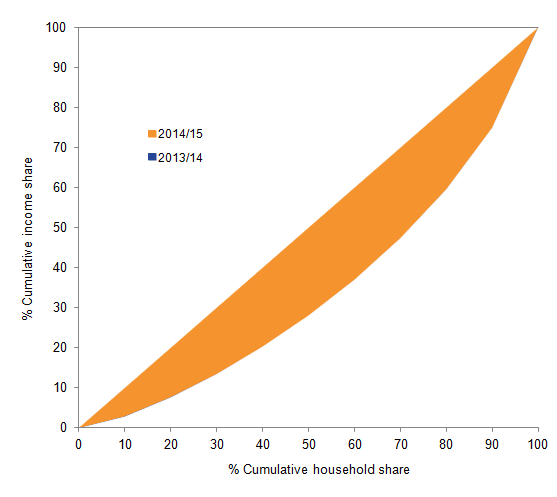
Another way of presenting income inequality is to compare income shares for different deciles or quintiles of the population. Figure C shows the proportion of aggregate income held by each decile. Overall there was very little change between 2013/14 and 2014/15.
Figure C: Percentage of equivalised disposable income held by each decile, 2013/14 and 2014/15
Source: Office for National Statistics
Download this chart Figure C: Percentage of equivalised disposable income held by each decile, 2013/14 and 2014/15
Image .csv .xlsSummary measures of income inequality
Gini Coefficient
It is possible to summarise a Lorenz curve in a single figure – a Gini coefficient. The Gini coefficient is probably the most commonly used measure of income inequality internationally and is effectively a summary of the differences between each household in the population and every other household in the population. Using the Lorenz curve, the Gini coefficient is calculated by taking the ratio of the shaded area and the area below the 45 degree line of perfect equality (the 45 degree line triangle). A distribution of perfectly equal incomes has a Gini coefficient of zero (or 0%). As inequality increases, and the Lorenz curve bellies out, so does the Gini coefficient, until it reaches its maximum value of 1 (or 100%).
One of the main strengths of the Gini is that it takes into account changes in relative incomes in all areas of the income distribution. It is always the case that an increase in the income of a household with an income greater than the median will lead to an increase in the Gini coefficient, as will a decrease in the income of a household whose income is below the median. The size of this increase in the coefficient will depend on the proportion of households that have an income between the median and that of the household whose income has changed. The Gini coefficient for disposable income in 2014/15 was 32.6%, compared with the 2013/14 value of 32.4%.
Table A shows that original income is more unequal for retired households than for non-retired households (Gini coefficients of 57.7% and 44.2% respectively). This is because the majority of those who are retired have little income from wages and salaries as they are not active in the labour market. In contrast, the Gini coefficient for gross income is markedly reduced among retired households (28.2%) and is smaller than the equivalent Gini coefficient for non-retired households (36.2%). This is primarily because of the addition of the state pension and pension credit. Inequality, as measured by the Gini coefficient, is lower for retired households at both the disposable and post-tax income stages than for non-retired households.
Table A (Reference Table 11): Gini coefficients of households, 2014/15
| Percentage | Original Income | Gross Income | Disposable Income | Post-tax Income |
| Non-retired households | 44.2 | 36 | 33.2 | 36.9 |
| Retired | 57.7 | 28.2 | 26.8 | 31 |
| All households | 50 | 35.8 | 32.6 | 36.4 |
| Source: Office for National Statistics | ||||
Download this table Table A (Reference Table 11): Gini coefficients of households, 2014/15
.xls (17.4 kB)In all Gini coefficients shown, income measures are equivalised using the modified-OECD scale. Strictly speaking, it could be argued that the equivalence scales used here are only applicable to disposable income because this is the only income measure relating directly to spending power. Since the scales are often applied, in practice, to other income measures, it is considered appropriate to use them to equivalise original, gross and post-tax income for the purpose of producing Gini coefficients. However, it is not felt to be appropriate to equivalise the final income measure because this contains notional income from benefits in kind (such as that from the NHS): the equivalence scales used in this analysis are based on actual household spending and do not, therefore, apply to such items as notional income.
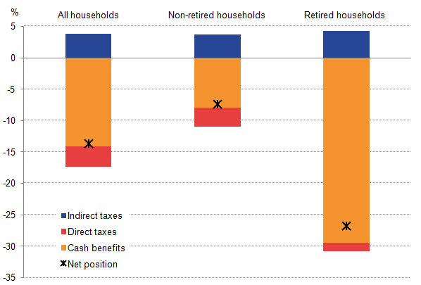
The effectiveness of taxes and benefits in reducing inequality can be investigated by looking at the changes in the Gini coefficients at each stage of the redistributive process. As illustrated in Figure D, cash benefits had the largest effect in reducing inequality of both retired and non-retired households, leading to a 29.5 and 8.0 percentage point reduction in the relative Gini coefficients, respectively. As stated above, the primary reason for the large effect on the inequality of incomes of retired households is the addition of income from the state pension and pension credits. Direct taxes reduced inequality for both retired and non-retired households by 1.4 and 3.0 percentage points, respectively. Indirect taxation increased inequality by 4.2 percentage points for retired and 3.7 percentage points for non-retired households. Measured in these terms, taken as a whole, in 2014/15 the UK tax and benefits system reduced inequality. Progressive direct taxes and cash benefits outweighed slightly regressive indirect taxation.
Figure D: Percentage point change in Gini coefficient due to cash benefits and taxes, 2014/15
Source: Office for National Statistics
Download this image Figure D: Percentage point change in Gini coefficient due to cash benefits and taxes, 2014/15
.png (10.9 kB) .xls (9.2 kB)
Other summary measures
The characteristics of the Gini coefficient make it particularly useful for making comparisons over time, between countries and before/after taxes and benefits. However, no indicator is completely without limitations and one drawback of the Gini is that, as a single summary indicator, it cannot distinguish between different shaped income distributions. For that reason, it is useful to look at this index alongside other measures of inequality. One such measure is the S80/S20 ratio, which is the ratio of the total income received by the 20% of households with the highest income to that received by the 20% of households with the lowest income. Another related measure is the P90/P10 ratio. This is the ratio of the income of the household at the bottom of the top decile to that of the household at the top of the bottom decile.
A relatively recently developed inequality measure, the Palma ratio, takes the ratio of the income share of the richest 10% of households to that of the poorest 40% of households. The idea behind using the Palma ratio is that middle 50% of households are likely to have a relatively stable share of income over time, and hence isolating them, should not lead to a substantial loss of information (Cobham & Sumner, 2013). Together these measures provide further evidence on how incomes are shared across households and how this is changing over time.
Figure E shows how each of these measures has changed over time in the UK, based on the effects of taxes and benefits on household income data.
Figure E: Change in Gini coefficient, S80/S20 ratio, P90/P10 ratio and Palma ratio for equivalised disposable income, all households, 1977 to 2014/15
Source: Office for National Statistics
Download this chart Figure E: Change in Gini coefficient, S80/S20 ratio, P90/P10 ratio and Palma ratio for equivalised disposable income, all households, 1977 to 2014/15
Image .csv .xlsThis chart shows that income inequality trends in the UK have been very similar on all 4 measures. Inequality of disposable income increased in the late 1980s and, to a lesser extent, during the late 1990s during periods of faster growth in income from employment, and fell in the early 1990s during a period of slower growth in employment income.
Since the turn of the millennium, changes in income inequality have been relatively small. In the early 2000s, income inequality fell. This was in part due to faster growth in income from earnings and self-employment income at the bottom end of the income distribution. Policy changes, such as increases in the national minimum wage, increases in tax credit payments, and the increase in National Insurance contributions in 2003/04 are also likely to have had an impact.
The most recent peak in income inequality was in 2006/07 or 2007/08 depending on the measure used. Since then there has been a slight fall in inequality on most measures.
Measuring inequality at the top of the distribution
There is particular public interest in looking at the incomes of the very richest households and how they relate to the rest of the population. However, as the effects of taxes and benefits data are based on a survey of 5,000 households, this means that any statistics for the top 1% (or 0.1%) of the distribution would be based on a small number of households and would not be sufficiently precise to draw accurate conclusions.
The best set of official statistics for looking at high income individuals is the Survey of Personal Incomes (SPI), produced by HMRC. However, the SPI does not cover individuals with personal incomes below the income tax personal allowance, and no attempt is made to estimate the numbers of people below this threshold or the value of their incomes.
One unofficial source of statistics which presents measures on the income share of the top 0.1% and 1% is the World Top Incomes Database, which contains figures for the UK developed by Sir Tony Atkinson.
Nôl i'r tabl cynnwys9. Coherence with other sources
This section presents a number of existing income and earnings measures that can be used to provide comparisons with data from the effects of taxes and benefits (ETB) release. It compares the income measures of the effects of taxes and benefits with Households Below Average Income (HBAI) figures published by the Department for Work and Pensions (DWP), before presenting comparisons with a broader range of income and earnings measures. The comparison with HBAI is the same as that provided in the previous release of this publication since no additional data are available.
Comparison with HBAI
DWP publishes analysis each year on household income in their publication Households Below Average Income (HBAI). The latest edition of this publication, including data for 2013/14, was released 25 June 2015. This release is based on data from the Family Resources Survey (FRS) and focuses on the lower part of the income distribution.
HBAI has a different focus from ETB, which is primarily focused on the redistribution of income through taxes and benefits across the income distribution. However, in order for both publications to be able to present a coherent narrative, some comparable statistics are presented in both bulletins.
The methodologies and concepts used for HBAI are broadly comparable to ETB, although there are some small but important differences. For example:
- ETB includes benefits in kind provided by employers (e.g. company cars) within income, but these are excluded from HBAI.
- HBAI includes certain benefits in kind provided by the state (such as free school meals and Healthy Start vouchers) within Before Housing Costs (BHC) income, which is otherwise equivalent to the ETB measure of disposable income. In ETB, these are included with other benefits in kind as part of final income.
- HBAI makes an adjustment for 'very rich' households using data from HMRC's Survey of Personal Incomes.
- ETB measures inequality on a household basis, whereas HBAI measures inequality on an individual basis.
HBAI is based on equivalised disposable household income being applied to each individual in the household, whereas ETB uses household level data. Over time, changes in household composition may have an impact on the comparability of the two series. In the analysis that follows, caution should be taken as this effect is not considered.
These differences in approach and the different survey sources mean that HBAI and ETB estimates can differ slightly from each other. However, historical trends are broadly similar across the two sources.
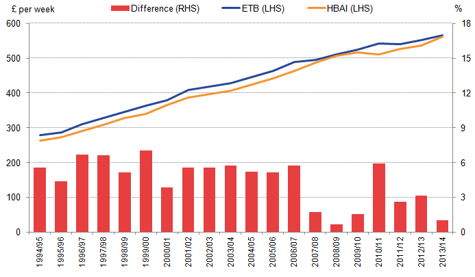
As HBAI provides an estimate of net weekly income (before housing costs) after adjusting for household size and composition, the closest comparator from the ETB release is the equivalised disposable income series. Over the twenty year period since 1994/95, the mean equivalised disposable household income from these two series has remained broadly similar across time. Since 2007/08, the two series have become even closer in level terms and were only 1.0% different in 2013/14 (Figure F), the most recent year for which HBAI data are available.
Figure F: Comparison of mean household ETB and HBAI nominal equivalised disposable (net BHC) income
Source: Office for National Statistics
Notes:
- Please note: Figure F was updated on 13/04/17 - previously referred to a median, this should have referred to the mean. This has been amended.
Download this image Figure F: Comparison of mean household ETB and HBAI nominal equivalised disposable (net BHC) income
.png (21.1 kB) .xls (27.1 kB)
ETB and HBAI also produce relatively similar estimates of the income distribution. In recent years, ETB has generally recorded lower disposable incomes than HBAI equivalised net income (BHC) in quintile one but higher in quintiles two to five. This was the case again in 2013/14, when median equivalised disposable household income in the ETB ranged from 0.9% lower than HBAI in the bottom quintile to 8.6% higher in the top quintile. These differences at the upper end of the distribution possibly reflect the variations in the measurement approach between ETB and HBAI mentioned above, such as the inclusion of employer benefits in-kind in ETB and the SPI adjustment in HBAI.
This similarity in estimates of the levels of income across the income distribution is also reflected in the growth rates for each group. Figure G shows the annual average growth rates of median equivalised disposable income for each quintile between 1994/95 to 2013/14. Across the two measures, the five quintiles grew at similar average annual rates. There was some disparity in the bottom two quintiles, with the ETB measure growing very slightly slower than the HBAI measure in the first quintile (4.0% compared to 4.1%) but stronger in the second (4.3% compared to 4.1%). The three top quintiles, however, grew at almost identical rates across the period.
Figure G: Compound average annual growth rates in median equivalised disposable household income by quintile, 1994/95 to 2013/14
Source: Office for National Statistics
Download this chart Figure G: Compound average annual growth rates in median equivalised disposable household income by quintile, 1994/95 to 2013/14
Image .csv .xlsComparison of the ETB income measure with other income and earnings measures
While the similarities between the ETB and HBAI income measures make this comparison relatively straightforward, it is also possible to compare components of the ETB income measure to other official statistics on earnings from employment.
The Average Weekly Earnings (AWE) measure is ONS’ lead indicator of short-term changes in earnings. AWE is the ratio of estimated total employee pay for the whole economy, to the total number of employees. The series is calculated from returns to the Monthly Wages and Salaries Survey (MWSS), to which there are 9,000 business respondents covering 13.8 million employees. The results are weighted to be representative of the UK economy as a whole, excluding the self-employed. As a consequence, it possible to compare the AWE with the value of average weekly earnings derived from the ETB. Figure H presents this comparison, and suggests that the two series have been very close, both in terms of levels and in growth rates, since 2007, although the gap has widened slightly in the financial year 2014/2015. The difference in the level of weekly earnings is less than 1% in most of the periods shown, however in the recent periods the difference between the two measures has increased, peaking at 2.3% in 2014 Q1 to 2014 Q4. The growth rates of the two series over this period were 15.0% in ETB, compared with 13.1% in AWE.
Figure H: ETB average weekly wages and salaries, four quarter moving average, and Average Weekly Earnings: £ per week

Source: Office for National Statisticsa
Download this image Figure H: ETB average weekly wages and salaries, four quarter moving average, and Average Weekly Earnings: £ per week
.png (18.6 kB) .xls (10.1 kB)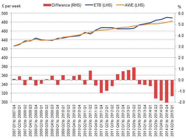
Finally, the aggregate movement in the ETB measure of equivalised household disposable income can be compared to a range of other statistics which capture average household incomes to differing degrees. Figure I compares average equivalised household income from ETB with three broadly comparable measures:
- EU Statistics on Income and Living Conditions (EU-SILC) – equivalised household disposable income: EU-SILC is the EU reference source for comparative statistics on income. It is coordinated by Eurostat and is collected jointly by ONS and DWP in the UK.
- Nominal GDP per household: This measure divides the total value of production and income in the UK economy by the number of households, so as to present the average value of income produced per household.
- Gross Disposable Household Income (GDHI) per household: GDHI per household is the average income available to households for spending or saving after income distribution measures have taken effect. It is based on the data for the household sector in the national accounts.
Figure I: A comparison of mean equivalised disposable household income to other income and earnings estimates
Source: Office for National Statistics
Notes:
- The ETB, nominal GDP per HH and GDHI per HH series are calculated on a financial year basis. The EU SILC series is calculated on a calendar year basis.
Download this chart Figure I: A comparison of mean equivalised disposable household income to other income and earnings estimates
Image .csv .xlsFigure I shows that the measure from the ETB release is broadly in line with other indicators over this period. In the years just prior to the downturn, the series showing the strongest income growth was the EU-SILC measure of income, but this has grown relatively weakly since 2009/10. Nominal GDP per household – which has recorded the strongest growth of these series since 1999/2000 – has grown at a weaker rate than the ETB average equivalised disposable income since 2005/06, while GDHI per household has followed a similar path to the ETB measure throughout the entire period.
Nôl i'r tabl cynnwys