1. Introduction
Office for National Statistics (ONS) is the UK’s largest independent producer of official statistics and its recognised national statistical institute. We are responsible for collecting and publishing statistics related to the economy, population and society at national, regional and local levels. We also conduct the census in England and Wales every 10 years. We hold a wide variety of microdata that are beneficial for evidence-based policy and advancement of research but are constrained by confidentiality concerns. One way to overcome this issue is the release of synthetic data in place of observed values as a method of statistical disclosure control for the public dissemination of microdata.
This working paper describes the outcomes from a small six-week project to investigate within ONS the demand and requirements for synthetic data, and to explore available tools and to demonstrate the ability to produce synthetic data for a particular user requirement. Existing tools to generate synthetic data were reviewed, and a use case implemented using the open source software R.
Synthetic data at ONS
This definition of synthetic data by the US Census Bureau aptly summarises what is meant by synthetic data:
“Synthetic data are microdata records created to improve data utility while preventing disclosure of confidential respondent information. Synthetic data is created by statistically modelling original data and then using those models to generate new data values that reproduce the original data’s statistical properties. Users are unable to identify the information of the entities that provided the original data.”
There are many situations in ONS where the generation of synthetic data could be used to improve outputs. These include:
provision of microdata to users
testing systems
developing systems or methods in non-secure environments
obtaining non-disclosive data from data suppliers
teaching – a useful way to promote the use of ONS data sources
ONS methodologists have recognised this as something that requires attention – but there has never been significant sustained effort in this area. There has been previous work in organising workshops in 2014 and 2015, work with the University of Southampton, and some potential tools have been explored but these have not been disseminated widely or put into a form that analysts can put into practice. This project was an initial step towards pulling together that previous work and developing a programme of research to develop methods for synthetic data.
There are many different types of synthetic data and methods with which to produce it. If synthetic data could be constructed with a high replication of structure and relationships, there are most likely to be some disclosure risks, which would require some research to explore. For example, there may be disclosure risks that may occur through chance or be based on perception.
Scope of the project
The main aim of the project was to deliver some user guidance for generating synthetic data, to review and possibly produce some initial software for doing this and to produce some synthetic data for a specific use case.
In this working paper we cover:
an overview of different types of synthetic data and propose a scale for high-level evaluation of quality (in terms of resemblance to real data) and disclosure risk accompanying synthetic datasets
statistical measures of similarity between synthetic and real datasets
review of several software tools for data synthetisation outlining some potential approaches but highlighting the limitations of each; focusing on open source software such as R or Python
initial guidance for creating synthetic data in identified use cases within ONS and proposed implementation for a main use case (given the timescales, the prototype synthetic dataset is of limited complexity)
a review of important references to work done to date in ONS, government, other National Statistical Institutes and across academia
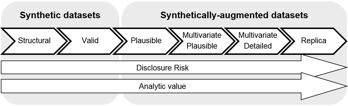
2. Synthetic dataset spectrum
We propose a high-level scale to evaluate the synthetic data based on how closely they resemble the original data, their purpose and disclosure risk (Figure 1).
At one end we define a purely synthetic dataset suitable for code testing with no ambition to replicate underlying data patterns and at the other end of the spectrum sits a dataset created by clever augmentation of the original, which aims to replicate the patterns contained within the original data source. Clearly, the latter carries extremely high disclosure risk and needs to be approached cautiously.
We also propose that the term synthetic data is used only for the first two levels on our spectrum to reflect general expectation of the term synthetic. A non-specialist audience does not expect any disclosure problems for synthetic data; synthetic records should be different from the real ones. Unfortunately, if an aim is to preserve fine multivariate distributions, then whole records are likely to appear in the synthetic dataset unchanged (even if generated from a model) and are therefore disclosive.
The later levels (3 to 6) are therefore referred to as synthetically-augmented datasets.
Figure 1: Synthetic dataset spectrum
Source: Office for National Statistics
Download this image Figure 1: Synthetic dataset spectrum
.png (33.4 kB)
Synthetic dataset
Synthetic structural
Preserve only the format and datatypes, that is, variable names should be preserved as well as their type (string, date, float and so on).
Contains only values present in the original (univariate) data.
Constructed based only on available metadata; values are generated from ad-hoc distributions and open sources.
To be used for very basic code testing, no analytical value, no disclosure risk.
Synthetic valid
Preserve the format and datatypes as detailed previously and ensure that a combination of variables per one record is plausible according to the original data (that is, no employed infants, unless they appear in the original data).
Constructed based only on available metadata; values are generated from open sources and distributions, which give values in a reasonable range (for example, age 0 to 100 years) but no attempt made to match the real distribution.
Produced dataset passes the sanity check (validation condition or edit rules) the real dataset would need to go through.
Missing value codes, errors and inconsistencies should be introduced at this stage should they appear in the original data.
Disclosure control evaluation is necessary case by case because sometimes even the range of plausible values is too disclosive (for example, date of birth in a longitudinal study).
To be used for advanced code testing, no analytical value, minimal disclosure risk.
Synthetically-augmented dataset
Synthetically-augmented plausible
Preserve the format and record-level plausibility as detailed previously and replicate marginal (univariate) distributions where possible.
Constructed based on the real dataset, values are generated based on observed distributions (with added fuzziness and smoothing) but no attempt made to preserve relationships.
Missing value codes and their frequency is to be preserved.
Disclosure control evaluation is necessary case by case, special care to be taken with names and so on.
To be used for extended code testing, minimal analytical value, non-negligible disclosure risk.
Synthetically-augmented multivariate plausible
Preserve the format and record-level plausibility as detailed previously and replicate multivariate distribution loosely for higher level geographies.
Constructed based on the real dataset, values are generated based on observed distributions (with added fuzziness and smoothing) and some relationships that are characteristic to the dataset at hand are retained.
Missing value codes and their frequency is to be preserved.
Disclosure control evaluation is necessary case by case.
To be used for teaching and experimental methods testing, some analytical value, high disclosure risk.
Synthetically-augmented multivariate detailed
Similar to the previous level but more effort made to match the real relationships (joint distributions), for example, in smaller geographies and household structure.
Disclosure control evaluation is necessary case by case.
To be used for teaching and experimental methods testing, some analytical value, very high disclosure risk.
Synthetically-augmented replica
Preserve format, structure, joint distributions, missingness patterns, low level geographies.
Constructed based on the real dataset, values are generated based on observed joint or conditional distributions, while de-identification methods are applied.
Disclosure control evaluation case by case is critical.
To be used in place of the real data, high analytical value, extremely high disclosure risk, likely to be only available in secure research facility.
Statistical measures of similarity
The following section outlines some potential methods of evaluating synthetic datasets against their observed counterparts. It discusses potential measures and provides examples of where they have been used, if applicable. Generally, similar evaluation methods can be applied whether the data are generated from available open source metadata, or created from observed microdata. That is, whether the data are “truly” synthetic (level 2 on the synthetic dataset spectrum) or synthetically-augmented (levels 3 to 6 on the spectrum). Synthetic datasets that only preserve the format and types of variables (level 1 on the spectrum) should not have their statistical properties evaluated, as they are not intended to have any. If the format of the data is correct then these data are appropriate for code testing. These kinds of synthetic data are not discussed further in this section.
The appropriate method used to evaluate synthetic data will depend on balancing user needs against disclosure concerns and resources available to data owners. The focus of this section, therefore, is on giving an accessible overview of evaluation methods, rather than on software package recommendations or precise mathematical formulation. For clarity, we refer to those responsible for the original observed data (and generating the synthetic data) as data owners, and those who will have access to the final synthesised data as data users.
It is likely that synthetic data users would like synthetic data to resemble the original data as closely as possible. The degree to which this is possible depends on the balance between user needs and the risk of disclosure. Generally, synthetic data that reflect higher levels of the spectrum will more closely resemble original data than lower level synthetic data. Careful consideration by the data owners should be given before releasing synthetic microdata, which preserve multivariate distributions with a high degree of accuracy.
On the other hand, a synthetic dataset must preserve some statistical properties of the original data for it to have any analytical value. First, the validity of the synthetic data needs to be evaluated (for example, ensuring no employed infants have been synthesised). Second, the key statistical properties should be compared to the original data to determine whether they have been retained.
Analysis of the synthetic data should yield similar estimates of the important statistical estimates as analysis of the original data (for example, group means, cell counts and correlation coefficients should be of similar magnitude in both datasets and the distributions of important variables should be similar). However, synthetic data may closely preserve some important statistical properties from the original data and fail to preserve others. Data owners should consult with users to decide which distributions and estimates are important for their purposes. Retaining these should be prioritised.
Simple methods of evaluating synthetic data against the original data include visual comparisons of important univariate distributions and calculating the relative or absolute differences in obtained estimates such as group means. More complex methods to evaluate, for example, multivariate distributions, may involve statistical modelling of both datasets and examining the differences in model parameters. Any kind of evaluation could involve the release of metadata detailing the degree of discrepancy between the synthetic and original data (example figures of dataset comparisons are given in the Resources and references section). Released metadata should inform users and analysts of how representative the synthetic data are of the original data.
Before evaluating synthetic data, there are some considerations that data owners should make:
where disclosure is a risk, data owners should balance the need for realistic data against real or perceived confidentiality infringements; it is not acceptable to release a synthetic dataset that could lead to a real or perceived risk of disclosure, in such circumstances, appropriate disclosure control methods should be applied before releasing statistics and data (see the Code of Practice for Statistics section on data governance T6.4)
released metadata should be detailed enough for end users to know how representative the synthetic data are of the original data, but not so detailed that the original microdata could be reconstructed
data users may require retaining some data errors to reflect real-life data (for example, invalid or missing data); errors can be retained or introduced on purpose when generating synthetic data, dependent on the use case
data users should be realistic about the number of multivariate distributions that can be accurately retained in the synthetic data, as the possibility of accurately retaining the entire multivariate structure of the original data diminishes as the number of variables in a dataset increase; when consulting with owners, users should ensure they focus on the few main relationships needed for their analysis
how to preserve string or text data is less well documented than numeric data and many users may not be interested in preserving names or specific address information; however, such information may be of interest to those whose aims include data linkage where such information can be used as data spines
metrics can be developed to compare the similarity of string data (for example, via string comparators); however, this is beyond the scope of the current section and its focus on statistical properties (evaluating synthetic string data is a topic for future research)
Univariate distributions
Important statistics and parameters from the synthetic and original datasets are calculated and compared. Comparisons will generally comprise graphical representations and/or examination of the descriptive statistics.
Categorical variables
For categorical data, owners can inspect the relevant tabular data (for example, cell counts) and/or visualise relative frequency distributions. Users may be interested in the differences between observed and expected counts in the case of n x 1 tabular data.
Continuous variables
When evaluating synthetic continuous data, owners may want to compare:
medians
means
quartiles or other quantiles
outliers or values at the extremes of the distribution (for example, top or bottom 5% of values)
measures of variability
Owners may also wish to calculate the relative percentage difference or absolute difference between these measures and consult with users to determine an acceptable level of difference.
Owners could examine whether point estimates from synthetic data fall within the 95% confidence intervals of the observed data (indicative of good fit), or the degree of overlap between the 95% confidence intervals of estimates obtained from the original and synthetic data. The larger the overlap, the more similar variables are likely to be. For example, observed survey data gives a population estimate for an area of 500,000, with the lower bound of the 95% confidence interval being 490,000 and the upper bound being 510,000. A point estimate from the synthetic data in the range 490,000 to 510,000 would be sufficient on the basis of 95% confidence intervals.
To visualise differences in (semi-)continuous data (for example, with a truncated distribution, or where “no code required” is included in the variable), users can plot histograms, cumulative frequency functions, or box plots. Raab and others (2016) recommend in Practical data synthesis for large samples (PDF, 336KB) that the owner of the data should visually inspect the marginal distributions of the synthetic data against the observed data as a minimum before releasing to users.
Multivariate distributions
Categorical variables
Multivariate distributions of categorical variables can be evaluated through use of frequency tables or contingency coefficients. Owners could examine the frequencies within the cells of a Variable A by Variable B (by Variable C and so on for more complex scenarios) for absolute or relative differences in the estimates between original and synthetic data. Joint distributions can also be visualised through mosaic plots.
Owners can calculate the Variable A by Variable B contingency coefficients for all variables of interest for both datasets. These can then be compared through the relative or absolute difference of each coefficient between the datasets. This can verify whether the relationships between main variables have been retained in the synthetic data.
Owners can also test the proportion of data in each cell in a contingency table between synthetic and observed data via z-scores. Here, the z-score is based on the relative size of a given category between the observed and synthetic data. The obtained z-scores can be squared and summed to give a chi squared measure of fit for the contingency table.
Model-based methods can also be applied to categorical variables, for example, logistic regression. Here, the user-defined model of choice is run on the original data and the synthetic data. The resulting logistic regression coefficients are then compared (either in relative or absolute terms). This approach could be extended to propensity score methods (typically for binary variables). Classes can be created based on propensity scores (for example, median split of scores, or K-groups from relevant quantiles), which determines whether the same proportion of records in the synthetic data fall into each class as in the observed data. For more information, see “Categorical variables” in the References and examples section.
Continuous variables
When a user wishes to preserve (some of) the multivariate structure of the observed data, a multiple regression model containing the important variables can be applied to the original data and then to the synthetic data. The obtained regression coefficients can then be compared. Again, this can be done in either absolute or relative terms, or the degree of overlap in the 95% confidence intervals can be examined.
Note that only the variables of interest should be included in this approach. Retaining the entire multivariate structure of the data becomes increasingly computationally problematic as the number of variables increases, and ultimately less informative as the models become over-fitted. For larger numbers of variables, data reduction techniques could be used to determine whether the same important features in the original and synthetic data have been retained. Categorical data could be submitted to multiple correspondence analysis and continuous data to principal component analysis. These techniques identify the most important dimensions within the data; both original and synthesised variables should yield similar dimensions.
For more information, see “Continuous variables” in the References and examples section.
Other considerations
Comparing synthetic data with unknown distributions
Some software packages allow observed sample survey data to be “scaled-up” into synthetic population-level data. In this case the relevant population distributions may be unknown. Bootstrapping procedures can be used as a method to evaluate the synthetic data where the population distributions are unavailable. Bootstrapping assumes the observed sample contains information about the population distribution. By resampling (with replacement) from the observed data multiple times, we can simulate the population distribution, and then compare the synthetic population to obtained estimates (for example, in terms of standard errors and confidence intervals surrounding an estimate).
Where synthetic sample data have been generated from observed data, but sample data are known to not conform to population distributions, weighting procedures can be applied to the synthetic data to yield population estimates as they would the observed data (weights themselves may also be generated synthetically).
For more information, see “Other considerations” in the References and examples section.
Multiple synthetic datasets
Some synthetic data generation methods and software packages involve creating multiple synthetic datasets, providing multiple replicants of the original data. Here, multiple synthetic datasets are pooled together for comparison. Users can calculate average summary statistics over their multiple synthetic datasets for whichever evaluation measures are deemed most appropriate. Average deviation from these estimates can also be calculated. For example, the mean difference (and variance) between the multiple synthetic Variable A and observed Variable A could be released as metadata. (Note that at this point that any bias in the data synthesis process may become apparent. If most or all synthetic data estimates over- or under-estimate the original data estimate there may be some systematic bias in the method used to generate data.)
Where synthesising categorical data across multiple synthetic datasets, a binomial distribution is built. From here, z-scores can be calculated for each cell in the table, which will indicate the relative size difference between the synthetic and observed values. Users could specify a z-score at which the difference between datasets is unacceptable, or extend this method to conduct a chi-squared goodness-of-fit test.
Summarising estimates from multiple synthetic datasets and comparing with the original data could, in principle, be applied to a number of the approaches outlined in this section.
For more information, see “Multiple synthetic datasets” in the References and examples section.
Geography
Geographies may be considered a special case of categorical variable if used for benchmarking in the synthesis process. Benchmarking here refers to the geographical level at which data are generated. For instance, an owner may aim to produce synthetic data at low geographical levels, which are then combined to create the final set, or they may aim to synthesise estimates at a high geographical level, which could then be analysed at lower levels.
The former approach has the advantage of producing more reliable estimates at lower levels, but the potential pitfall is that if there is some bias in the synthesis process, errors may quickly compound to produce unreliable aggregate estimates at higher levels. The latter approach potentially averts the compounding issue, but may produce unreliable estimates at the lower levels due to data smoothing. Users should consider the level at which to evaluate the data (lower levels, higher levels or both), informed by the method used.
For more information, see “Geography” in the References and examples section.
Verification servers
External users without access to the original dataset cannot run their own evaluation statistics. Researchers may find it difficult or impossible to determine the representativeness of the synthetic data based on information released about the observed data (such as aggregates or metadata). One solution to this is verification servers, which have the potential to provide automated feedback on the accuracy of synthetic data analysis.
Verification servers have access to both the synthetic and observed data. The general process involves the external researcher analysing their data. This user then submits a summary of their analysis to the verification server (for example, regress Variable A on Variable B and Variable C). The server then performs the analysis on both the synthetic and original datasets. It then returns the overlap of confidence intervals of the synthetic and observed data.
A second approach is for users to specify, for example, a minimum value for an estimate that is of analytical interest. The server then returns whether this condition is satisfied. This approach may be preferred when the dataset contains a large number of records, giving narrow confidence intervals surrounding a point estimate. The analyst then can determine how representative the synthetic data are for their purpose.
Designers of verification servers must be cautious – such servers have the potential to leak confidential information. Snoopers could submit queries (perhaps used in conjunction with other information) that allow them to ever more accurately estimate confidential information. Limiting the types of queries or giving only coarse responses to user queries may reduce these concerns.
For more information, see “Verification servers” in the References and examples section.
Releasing metadata
The choice of metadata to release will depend on its structure and expected final use. Owners of original data will need to balance what is critical to understanding the representativeness of synthetic data with what is reasonable to produce, given available resources. For example, for a dataset containing hundreds of variables it may not be feasible to release detailed estimates for every variable and certainly not for every combination of variables. It may be pragmatic only to focus on variables that contribute to critical outputs, or perhaps specifically requested by users. For datasets containing fewer variables, it may be possible to release more detailed metadata.
Similarly, the choice of metadata is limited by the level at which data are synthesised. Synthetic data that have a higher level on the synthetic dataset spectrum – where care has been taken to preserve many multivariate relationships – have the potential for more detailed metadata to be released, compared with data that have a lower level on the spectrum with only univariate distributions preserved. Where data have been synthesised from open source aggregate or metadata, the obtained synthetic data can only ever be evaluated against those available parameters.
The choice of whether to release absolute or relative differences (or both) between synthetic and observed data is also a consideration. Consider a case where an estimate obtained from a synthetic data variable is 0.1 and the same estimate from the original data is 0.05. The synthetic data has produced an estimate twice the size of that obtained from the observed data whereas the absolute difference is 0.05. This may be trivially small or unacceptably large depending on the interpretation of that estimate. Subject matter experts may be best placed to provide guidance on the most informative types of metadata.
Where multiple synthetic datasets have been produced, it is possible to release some indicator of the variability between the datasets, or discrepancy between estimates. For example, the metadata could contain the number of times data were synthesised, the range of a particular estimate over the multiple datasets and a measure of its variability. These metadata could be released even if the data are synthesised multiple times but only one dataset is made available.
Nôl i'r tabl cynnwys3. Software and tools
When choosing the right software package or tool we should consider not only the specific task for which it is needed but context of the whole project. This might limit the choice to specific environment (for security reasons), programming language or open licence software.
This chapter provides an overview of several software solutions that are available across most platforms currently used in Office for National Statistics (ONS). This includes web-based tools (Mockaroo, random.api, yandataellan), R packages (synthpop, simPop, sms) and Python packages (Faker).
The following sections contain an overview of each package, a table summary based on main criteria and a decision flowchart to find the right tool based on purpose.
Overviews of synthetic data software
Web-based tools
There are several websites or standalone downloadable tools that allow users to generate synthetic data for code testing purposes. The data are generated either from specified simple distributions (numeric) or from the provider’s database (for example, names, addresses). Limited dependencies between variables can be specified. Free versions of the software sometimes restrict the number of generated records.
Examples of such web applications are mockaroo.com, random.api, and yandataellan.com. Similar standalone free to use software is Benerator.
These tools are best suited for synthetic data at the lowest level of the synthetic dataset spectrum: synthetic structural or valid.
Advantages of web-based tools:
no prior programming knowledge assumed, so anybody can generate a dataset very quickly
a large number of variable types are implemented as standard; data types include first and last names (and email addresses based on these names); numerical data following predefined distributions (for example, random, normal, exponent); addresses; continuous numerical data; predefined ranges for numerical data to simulate custom categorical data
users can specify a percentage of records within each variable to be left blank to simulate missing data
produces common data files (for example, CSV)
Disadvantages of web-based tools:
there are no “out-of-the-box” dependencies (for example, age and marital status could be inconsistent for large numbers of records)
custom dependencies are difficult to implement (if possible), for example, Mockaroo offers custom formula input using Ruby scripting to somewhat attenuate the synthesis of inconsistent data; however, if the user requires large numbers of dependencies, inputting formulas may become cumbersome and defeat the purpose of a product with speed and no coding knowledge advantages
Synthpop R package
Synthpop is a package for synthesising data from an existing (observed) dataset. It is freely available as an add-on to R software, so prior knowledge of R is needed. An initial variable is synthesised using random sampling with replacement before classification and regression trees are applied to generate the rest of the synthetic dataset. Variables are synthesised sequentially, preserving their conditional distributions. Different regression methods (such as linear and logistic) are offered. Thus, synthpop preserves the essential statistical properties of the data; as such synthetic data can resemble observed data very closely (which has disclosure implications for publicly available datasets). It would be therefore a tool of choice for the higher levels on the synthetic dataset spectrum: synthetically augmented multivariate up to replica.
Functions:
a synthetic dataset using default settings can be produced using a single command
users can synthesise all data or a subset of selected variables
the minimum size of the “minibucket” in the terminal classification and regression tree model can be customised (useful for disclosure control); Gaussian kernel smoothing can also be applied to mask unusual values
missing values can be synthesised; where variables have multiple types of missing values (that is, where data are missing for different reasons), they can be modelled separately
users can add labels to variables, making it clear that the dataset is synthetic
the selection of predictors used to synthesise target variables can be customised
rules can be implemented to stop the synthesis of nonsense data
the original and synthesised datasets can be compared within synthpop to assess whether essential statistical properties have been preserved using many of the methods described previously
Advantages of Synthpop R package:
adaptable “syn” function with many built-in options (choices of models, predictors)
once the models have been fitted, synthpop can produce any number of records by making more or fewer draws from said models using “k =” (though R can have memory constraints)
capable of generating data with no preserved relationships for categorical or numeric data, or closely maintaining relationships in the cases of few variables; models can be simplified to directly determine which variables are dependent on which (for example, all variables are related to age to prevent married four-year-olds, working 90-year-olds and so on)
in-built disclosure control function to remove unique records in the synthetic dataset that represent real records in the original dataset
models (trees) can also be simplified by raising the size of “minibuckets”, when classifying observations into groups or “buckets”, groups of this size or smaller are not differentiated any further; the larger these buckets, the less likely synthpop is to reproduce unique (disclosive) records
Disadvantages of Synthpop R package:
classification trees are prone to over fitting, maintaining all relationships is unlikely to be possible in cases of more than say 10 variables, depending on number of categories, complexity of relationships and so on
it has limited functionality for text variables – it does not add noise or fixed errors to text variables and does not create new text strings (names, addresses) but rather draws from existing values found in the real data; if direct identifiers were held and were sensitive, synthpop would reproduce the same sensitive values; if first names and last names were stored as two separate variables, synthpop would draw from exiting values independently, so that new full names may be produced, but first and last names would be directly reproduced from the data
For more information, see “Synthpop R package” in the References and examples section.
SimPop R package
SimPop is a package for synthesising data from an existing (observed) dataset. SimPop will generate a simulated population from observed sample data combined with geographical census macrodata. It is freely available as an add-on to R software, so prior knowledge of R is needed. Synthetic data are generated sequentially.
SimPop creates household structures from observed data (so not as to create unobserved, unrealistic households) via resampling. Then categorical variables are generated. These are allowed to have non-observed relationships to households, as the sample is unlikely to capture all possible (reasonable) relationships in the population. Users can also take into account within-household relationships when simulating categorical variables. Finally, continuous variables are generated.
Data generated by this package usually fall into the middle of the synthetic dataset spectrum: synthetically-augmented multivariate.
Functions:
SimPop uses multiple techniques in a stepwise fashion to create synthetic data (iterative proportional fitting, replication, modelling, simulated annealing)
default order of data synthesis is recommended, but this can be modified (simPop generates categorical variables before continuous variables; users can reverse this process)
users can apply corrections to age variables (Whipple, Sprague indices; corrects for over-reporting of ages ending in 5 or 0)
can simulate geographical regions at the smallest level as those areas known in the data
multiple methods for generating categorical variables are available: multinomial logistic regression, random draws from the conditional distribution or via classification trees
likewise, multiple methods are available for continuous data: creation of multinomial categories and sampling from those categories; via regression-based methods adding a random error term
initial synthetic data will not necessarily perfectly match the marginals of the observed data; if additional accuracy is required, users can post-calibrate the synthetic data via data perturbation (that is, moving households into different areas to find a better match with the observed marginals)
data utility according to preserved univariate and multivariate distributions is assessed at the end of the process; results of regression models applied to the original dataset are compared with results obtained when the same models are applied to the synthetic dataset
Advantages of SimPop R package:
SimPop handles complex data structures such as individuals within households
processing speed is fast due to ability to use parallel CPU processing
marginal distributions can be well preserved as they are used in the synthesising process
Disadvantages of SimPop R package:
- it has limited functionality for text variables – it does not add noise or fixed errors to text variables and does not create new text strings (names, addresses) but rather draws from existing values found in the real data
For more information, see “SimPop R package” in the References and examples section.
Sms R package
Sms is a package specifically for simulating small area population microdata. Sms combines individual-based datasets with census data. Individual data are randomly (with replacement) selected from a database and evaluated against the profile of a geographical area iteratively. This replaces individual records until small area constraints are satisfied. This procedure produces microdata for regions based on observed data and census macrodata. The more overlap between dataset and census variables, the better fit can be achieved.
This package is best suited for synthetic data at the higher levels of the synthetic dataset spectrum: synthetically augmented multivariate up to replica.
Advantages of sms R package:
it can create population-level datasets based on sample data
marginal distributions can be well preserved as they are used in the synthesising process
Disadvantages of sms R package:
the R implementation of this method does not deal with household and individual constraints at the same time
the simulated records are copied with minimal modification, which may lead to disclosure issues and low variability
For more information, see “Sms R package” in the References and examples section.
Faker Python package
Faker (or previously fake-factory) is a Python package that generates fake data. Its primary purpose is for code testing for developers.
Datasets created by this package are at the lowest level of the synthetic dataset spectrum: synthetic structural or valid.
Functions:
it can generate fake identifiers (name, address, email, date of birth) in several different languages
other variables can be simulated using bootstrapping from existing database or using user-specified distributions
export into desired file format achieved through usual Python functions
it can be used as part of a custom script (for example, adding fuzziness – fuzzywuzzy package)
Advantages of Faker Python package:
free and open-source
easy integration into custom code; you can use “seed” to make the generating process reproducible
Disadvantages of Faker Python package:
it requires knowledge of Python – users are expected to write their own wrapper to put the required variables together
Great Britain addresses have the right format but are made up (that is, non-existent postcodes, street names and so on)
the identification variables cannot be related for one record (for example, name and email address are obvious mismatch)
no transparent documentation about how exactly the data are generated
no default way to preserve relationships between variables
For more information, see “Faker Python package” in the References and examples section.
| Requirement | Software | ||||
|---|---|---|---|---|---|
| SimPop (R package) | Synthpop (R package) | Sms (R package) | Web-based tools (For example, Mockaroo) | Faker (Python) | |
| Creates synthetic data from an observed dataset | Yes | Yes | Yes | Creates file based on user input | Creates file based on user input |
| No "nonsense data" (for example, working children) | Yes | Yes | Yes | Difficult to achieve (or use post-processing) | No (manually or post-processing) |
| Categorical variables | Yes | Yes | Yes | Yes user-defined | Yes from custom DB |
| Numerical variables | Yes | Yes | Yes | Yes user-specified distribution | Yes |
| String data (For example, add controlled amount of noise to text strings for matching) | NA treated as categorical, no noise | NA treated as categorical, no noise | NA treated as categorical, no noise | Yes For example, generate first/last name, email addresses | Yes (add noise using fuzzywuzzy) |
| Admin-type data (may be useful for linking) | Yes | Yes it has a pool of names, addresses and so on. | |||
| Small geographical area estimation | Yes | No | Yes | No | No |
| Requires additional macro-data (for example, large geographical data from census) | Yes | No | Yes | No | No |
| Scales data to create a population-level dataset | Yes | No | Yes | No | No |
| Preserve marginal distributions | Yes | ||||
| Preserve conditional distributions | Yes, with processing or memory limitations | ||||
| Requires additional software (for example, R) | Requires R | Requires R | Requires R | No | Python / R |
| Preserve clustered data structures (for example, households) | Yes | No | No | No | No |
| Disclosure control tools | Yes | NA totally fabricated data | NA (no input microdata) | ||
| Missing data | Yes Missing structure of original data reflected in output | Yes Multiple types of missingness can be generated | No | Yes Users specifies percentage of each variable to be left blank | No (manually or post-processing) |
| Data generation method | Iterative Proportional fitting | Classification and regression trees | Combinatorial Optimisation | NA | bootstrapping & drawing from specified distribution |
| Localized to UK | NA | NA | NA | Yes | Yes but unreal postcodes |
Download this table Table 1: At-a-glance synthetic data package features
.xls .csv
Figure 2: Software decision flowchart
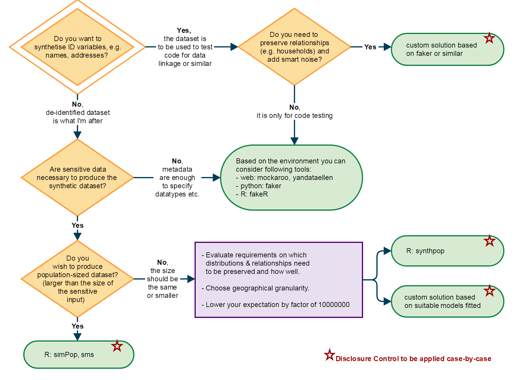
Source: Office for National Statistics
Download this image Figure 2: Software decision flowchart
.png (319.9 kB)
4. Case study
This case study explored one of the main use-cases identified for creating a synthetic dataset. The aim was to construct a synthetic data version of sensitive microdata held in the Office for National Statistics (ONS) Secure Research Service (SRS). The main reason is for easing the use of securely held data by allowing researchers to familiarise themselves with the format and structure of the data, and to test code, before accessing the data in the real secure environment. This will save the researchers time, as they can develop code in advance and be confident that it should (broadly) work on the real data when they get access. This gives them more time for analysis on the real data, and therefore better outcomes.
Labour Force Survey microdata
The Labour Force Survey (LFS) is the largest household survey in the UK. The LFS is intended to be representative of the UK, and the sample design currently consists of around 37,000 responding households in every quarter. The quarterly survey has a longitudinal design such that households stay in the sample for five consecutive quarters (or waves), allowing comparisons to be made over time (for more information, see About the Labour Force Survey). Its main purpose is to provide information on the UK labour market, which can then be used to evaluate and develop labour market policies.
LFS datasets are included amongst many datasets held and made available as part of the ONS SRS. It is one of ONS’s most popular microdata products and accounts for most visits to the SRS. The aim is to produce a synthetically augmented plausible (level 3) version of the LFS that could be provided to new researchers before their first travel to the secure laboratory, ultimately saving them time spent travelling to and from the secure data laboratory and allowing them to test code prior to arrival, as well as using space and processing resources within the SRS more efficiently. The important feature of such a synthetic dataset is that it reflects the actual LFS data in terms of the variables it contains and the data held – though importantly, is also non-disclosive. This would mean the synthetic version could be publicly available without license restrictions.
Note that a teaching file containing 12 variables is freely available already on the UK Data Service webpage. The user guides for the LFS (PDF, 32.7KB) are also freely available.
Approach
In this proof of concept, the aim was to synthesise a core subset of variables of the most recent LFS survey (Quarter 2 (Apr to June) 2017, the most recent available at the project start). The output dataset should correspond to level 3 of the suggested synthetic dataset spectrum, that is, focusing on record-level plausibility. For some variables (specified in Table 2), another aim was to preserve national-level aggregates and simple dependencies, including age appropriate economic activity (young respondents in education, middle aged more likely to work, older respondents more likely to be retired) and occupations, industry, income listed only for respondents in work.
Working through the decision flow-chart (Figure 2) with the aim of reproducing the securely held LFS microdata: we did not have an interest in synthesising direct identifiers, though we did require access to the sensitive data to preserve inter-dependencies in the data, such as the relationship between age and economic activity. We prefer to match the number of records available in the secure environment, rather than producing a larger population size version, which would exaggerate the sample sizes available and inflate the processing time required. Given these requirements, we use R, including the open source Synthpop package, and open datasets (for example, lookups from Open Geography Portal) to achieve this. We also required access to the original microdata, though alternative approaches would still be possible without direct access. The Synthesising using CSV input code, and copy of the input file for 22 variables are both available here. The generated LFS data can be made available on request.
| Variable name | Description | Variables it depends on | Short description of model used (dependency specs) | Resources required (that is, summary stats, regression coefficients, open data) |
|---|---|---|---|---|
| Geographic variables: | ||||
| OA11 | 2011 census Output Area | -- | uniform distribution | ONS geography lookups (list of possible values) |
| OAC11 | Census Output Area code | OA11 | deterministic | ONS geography lookups |
| OSLAUA9D | 9-digit local authority district | OA11 | deterministic | ONS geography lookups |
| URESMC | Region of usual residence | OA11 | deterministic | ONS geography lookups |
| CTRY9D | Country (9 Digit) | OA11 | deterministic | ONS geography lookups |
| GOR9D | Region (9 Digit) | OA11 | deterministic | ONS geography lookups |
| Demographic variables: | ||||
| AGES | Age band | --- | Random sampling from original data | Original data |
| AGE | Age in single years | AGES | Draw from Classification Tree model (in Synthpop) | Original data |
| AGEDFE | Academic age at school end of year | AGE | Draw from Classification Tree model (in Synthpop) | Original data |
| AGEEUL | Age bands (LFS End user license version) | AGE | Draw from Classification Tree model (in Synthpop) | Original data |
| SEX | Sex | AGES | Draw from Classification Tree model (in Synthpop) | Original data |
| MARSTA | Marital Status | AGES SEX | Draw from Classification Tree model (in Synthpop) | Original data |
| ETHUKEUL | Ethnic group (EUL version) | AGES SEX | Draw from Classification Tree model (in Synthpop) | Original data |
| Labour market: | ||||
| ILODEFR | Economic activity (ILO definition) | AGES SEX | Draw from Classification Tree model (in Synthpop) | Original data |
| INDS07M | Industry (1 digit) | AGES ILODEFR | Draw from Classification Tree model (in Synthpop) | Original data |
| ICDM | Industry (5 digits) | AGES INDS07M | Draw from Classification Tree model (in Synthpop) | Original data |
| SC10MMJ | Occupation (1 digit) | AGES INDS07M | Draw from Classification Tree model (in Synthpop) | Original data |
| SOC10M | Occupation (4 digits) | AGES SC10MMJ | Draw from Classification Tree model (in Synthpop) | Original data |
| OYSOCC | Occupation same as 12 months ago | AGES SC10MMJ | Draw from Classification Tree model (in Synthpop) | Original data |
| Design weights: | ||||
| PWT17 | Sampling weight | AGES SEX | Draw from Regression Tree model (in Synthpop) | Original data |
| Pay and Benefits: | ||||
| BANDN | Net income (banded) | AGES SC10MMJ | Draw from Classification Tree model (in Synthpop) | Original data |
| NET99 | Net income | AGES BANDN | Modelled missing/non-missing, random draw for non-missing values | Original data (Could be applied with missing/non-missingness and list of observed values) |
| BENFTS | Claiming benefits | AGES BANDN | Draw from Classification Tree model (in Synthpop) | Original data |
| Education variables: | ||||
| DEGREE71 | 1st degree held | AGES INDS07M | Draw from Classification Tree model (in Synthpop) | Original data |
| DEGREE72 | 2nd degree held | AGES DEGREE71 | Modelled missing/non-missing, random draw for non-missing values | Original data (Could be applied with missing/non-missingness and list of possible values) |
| DEGREE73 | 3rd degree held | AGES DEGREE72 | Modelled missing/non-missing, random draw for non-missing values | Original data (Could be applied with missing/non-missingness and list of possible values) |
| DEGREE74 | 4th degree held | AGES DEGREE73 | Modelled missing/non-missing, random draw for non-missing values | Original data (Could be applied with missing/non-missingness and list of possible values) |
| DEGREE75 | 5th degree held | AGES DEGREE74 | Modelled missing/non-missing, random draw for non-missing values | Original data (Could be applied with missing/non-missingness and list of possible values) |
Download this table Table 2: Summary of modelled variables by groups
.xls .csvA dataset of 88,801 records was produced, the same number as in the secure version of the data. It included 22 characteristics and six geographic variables. The characteristic variables were generated from statistical models based on the real data. As a special case, the geography was generated separately and at random.
The geographic information can act more independently than the characteristic variables, without ever producing impossible record-level combinations, and as the main variable in identifying records or disclosure risk, it would be preferable for geographic information to not closely match those of the real records.
The lowest level of geographic information (census Output Area, average of 300 residents) was chosen at random from all possible output areas, then the corresponding higher geographies from the census geography hierarchy were added. By synthesising geography in this way synthetic records have a very low probability of having a matching location with any real record, but no geospatial relationships were preserved in the data.
Region data could realistically be included in the modelling if desirable, but lower geography levels like Middle layer Super Output Area (MSOA, approximately 35,000 categories) would require much more involved modelling and would more closely correspond to level 5 of the synthetic dataset spectrum, which is not intended here.
The characteristic variables were created using either classification trees (for continuous variables) or regression trees (for categorical), which are the defaults in the Synthpop package (Breiman 1984). These tree-based methods make predictions based on specific splits or “branches” of the data, for example, when using age to predict marital status, the model will find that the subset of data where age is below 16 years will very often be “single”, whereas the subsets of data where age is over 85 years is more likely to be “widowed”.
The process will try many different possible splits and chooses one that creates the most homogenous groups possible (try to group the “single” records together, the “widowed” records, and the “married” records). Once the tree model has been formed, this can be used to generate new data based on the relationships found.
Based on the predictor values, the software will check which subgroup the new synthetic data belong to, for example, based on an age value of 45 years, which is part of the group that includes ages 36 to 48 years, 80% of this group are “married”, and 20% are “single”; a random draw is made from the observed values in this group so the record receives a value of “married”. These tree-based methods are simple to apply and contain a random element, so records are not directly reproduced, though they are prone to over-fitting and can be computer intensive.
To restrict computational requirements, each variable had a maximum of two predictors, though more could have been used in cases of variables with few categories. Synthpop defaults to using every available variable in the models, which is untenable for moderate or large datasets with several hundred variables, without using considerable computing power. Versions with fewer categories were used as predictors rather than the full detail (for example, one-digit occupation rather than four-digits). Using much more detail in predictors complicates the modelling and often loses information when related categories are modelled independently, particularly in hierarchical variables. In some cases, the resulting models can unnecessarily be based on very few observations within subgroups.
The underlying microdata were used in creation of this synthetic data, though if this was not available a more limited model could be created using only the possible levels or categories of each variable, for example, univariate frequency tables for each variable, though this would make it harder to maintain relationships between variables and avoid illogical combinations (likely to be a level 1, synthetic structural dataset).
Choosing predictor variables may be a difficult aspect to scale up to larger datasets, as this was done manually in this case, and requires knowledge of the data. Closely related variables were used in prediction. In particular, values of occupation, industry, and income should be valid for those who are economically inactive. This may be harder to achieve if many variables are inter-related. Grouped age was used as a universal predictor. The others were put into categories and a tree-like structure was used to preserve as many important relationships as possible with the fewest predictors: economic activity predicted industry, industry predicted occupation and education, and occupation predicted income.
Many variables had high levels of missingness, usually because the questions do not apply to all respondents. In cases like these, preserving the missingness and structure of the variable was more important than any multivariate relationships (which may be highly volatile depending on the survey sample). These variables (with less than 80% responses missing) were simplified into missing or non-missing before the synthesis, so only a binary presence or absence indicator was modelled. Where the variable should be non-missing, a value was chosen at random from the possible categories.
Overall, we have produced a non-disclosive synthetic version of a subset of the Labour Force Survey, that can be made available outside of a secure environment. It was produced based on the real data, using draws from statistical models (CART, classification and regression trees) without replicating the real records. It was intended to maintain only basic properties of the data on the most important variables and avoid record-level implausibility or nonsense values (level 2 to 3 on the synthetic dataset spectrum). Further work is needed to extend this beyond the main variables and closely maintain relationships found in the data (levels 3 and over).
Summary of steps involved
Choose data to be synthesised, and purpose of the synthetic data that will be produced.
Familiarise with the data, and which variables are the highest priority for the output.
For high priority variables, select a small number of predictors that are most relevant or have the most important relationships to preserve.
For low priority variables, select a universal indicator, such as age, which may have some predictive power for a wide range of variables; if none seem appropriate, use no predictors.
For low priority variables with high levels of missingness, replace with a binary missingness indicator, and save the possible categories.
Input the data and the chosen predictors into the Synthpop process.
Replace the binary indicator variables with randomly chosen categories, where the synthesised variable is non-missing.
Randomly select a geographical area for each record, from all possible areas; if the data contain multiple geographies, select at the lowest geography level and attach the corresponding larger areas.
5. Conclusion
Wide access to microdata is beneficial for advancement of research and evidence-based policy but it is often constrained by confidentiality concerns. Office for National Statistics (ONS) has explored synthetic data techniques to allow for the release of high-quality microdata without compromising confidentiality. This pilot project has delivered some user guidance for generating synthetic data, review of available software for generating synthetic data, and a detailed description of data synthesising for a specific use case. Our work also highlighted the limitations and challenges in the process of creating synthetic data.
Continued research in these areas will help to increase the quality and acceptance of using synthetic data for disclosure control and for research purposes. The next step of the research is to extend the guidance to cover more available tools and use cases. In addition, an extension of the prototype synthetic Labour Force Survey (LFS) dataset to include all characteristics for public usage is desirable.
Nôl i'r tabl cynnwys7. Resources and references
Government Statistical Service and Government Social Research guidance
GSS/GSR Disclosure Control Guidance for Tables Produced from Administrative Sources (published October 2014)
Regarding methods of statistical disclosure control, the guidance mentions (on page 25) "An alternative option is to create a synthetic dataset which maintains all the properties of and relationships in the true dataset. From these data, non-disclosive tables can be created."
ONS use cases
A synthetic data file produced from survey data in 2011 was developed for an Italian record linkage course, which is linked to from the Eurostat website.
Other use cases
Arrangements for access to national disease registration data held by Public Health England (published September 2017) – this guidance note mentions that Public Health England (PHE) supports such data access in two ways, and other options, such as a secure safe haven space and a cancer data model, containing synthetic or perturbed data were planned.
Alfons and others(2011), Synthetic Data Generation of SILC Data (PDF, 5MB) – this paper relates to synthetic data generation for European Union Statistics on Income and Living Conditions (EU-SILC).
Barrientos and others (2017), A Framework for Sharing Confidential Research Data, Applied to Investigating Differential Pay by Race in the US Government
Statistical measures of similarity
Multivariate distributions
Categorical variables
Diagnostic Tools for Assessing Validity of Synthetic Data Inferences
Voas and Williamson (2000), An evaluation of the combinatorial optimisation approach to the creation of synthetic microdata – this paper details the z-score approach.
See also the reference to Alfons and others (2011) under “Other use cases”.
Continuous variables
Drechsler and others (2008), Comparing Fully and Partially Synthetic Datasets for Statistical Disclosure Control in the German IAB Establishment Panel
See also the reference to Barrientos and others (2017) under “Other use cases”.
Other considerations
Comparing synthetic data with unknown distributions
Namazi-Rad and others (2014), Generating a Dynamic Synthetic Population – Using an Age-Structured Two-Sex Model for Household Dynamics
More information is also provided in the sms documentation.
Multiple synthetic datasets
More information is provided in the Synthpop documentation.
See also the reference to Voas and Williamson (2000) under “Categorical variables”.
Geography
Huang and Williamson (2001), A comparison of synthetic reconstruction and combinatorial optimisation approaches to the creation of small-area microdata
Verification servers
McClure and Reiter (2012), Towards Providing Automated Feedback on the Quality of Inferences from Synthetic Datasets
Vilhuber and Abowd (2015), Usage and Outcomes of the Synthetic Data Server
See also the reference to Barrientos and others (2017) under “Other use cases”.
Software and tools
Synthpop R package
White paper: Synthpop: Bespoke Creation of Synthetic Data in R was published in October 2016 in the Journal of Statistical Software. The Synthpop R package is available to download.
SimPop R package
White paper: Simulation of Synthetic Complex Data using simPop was published in August 2017 in the Journal of Statistical Software. The SimPop R package is available to download and an International household survey use case is also available.
Sms R package
White paper: sms: An R Package for the Construction of Microdata for Geographical Analysis was published in November 2015 in the Journal of Statistical Software. The sms R package is available to download.
Faker Python package
For more information, see Faker: package documentation, example usage.
Labour Force Survey
Information about the Labour Force Survey, including why the study is important, what is involved in the study and how the information is used, is available. More information about the Labour Force Survey is also available from the Health and Safety Executive.
Academic references
Breiman L (1984), Classification and Regression Trees, New York: Routledge
Martin and others (2017), Creating a synthetic spatial microdataset for zone design experiments
Raab and others (2016), Practical Data Synthesis for Large Samples
Voas and Williamson (2000), An Evaluation of the Combinatorial Optimisation Approach to the Creation of Synthetic Microdata
SYLLS synthetic longitudinal data spine (published 16 October 2017)
Synthetic Data Vault online article with a link to a paper (viewed on 3 October 2017)
Research from other National Statistical Institutes
Austria: Synthetic Data Generation of SILC Data by Alfons and others (2011) – an example of how to create and evaluate synthetic data.
New Zealand: Graham and others (2008), Methods for Creating Synthetic Data
New Zealand: Synthetic unit-record files (SURF)
US: Jarmin and others (2014), Expanding the role of synthetic data at the US Census Bureau
US: Vilhuber and Abowd (2015), Usage and outcomes of the synthetic data server
US: See also the reference to Barrientos and others (2017) under “Other use cases”.
Courses, conferences and events
Generating synthetic microdata to widen access to sensitive data sets: method, software and empirical examples (first link on page 4 – abstract only), Dr Beata Nowok, Edinburgh University, Government Statistical Service Conference, Birmingham, September 2015.
Generating synthetic data in R: Session 1 – Introduction and background, held on 22 March 2016 in Edinburgh. A course outline for sessions 1 and 2 is available.
Nôl i'r tabl cynnwys