1. Abstract
With the increasing availability of extremely large datasets of price and expenditure information, the price statistician faces a new set of challenges. Over the past few years, new methods have evolved for compiling price indices from such data sources. The analysis in this paper builds on previous Office for National Statistics (ONS) research into web scraped data (Breton et al., 2015; Breton et al., 2016), focusing on a dataset of clothing prices scraped from retailer's websites.
Clothing prices are typically accompanied by unique problems in measurement, due to the fast paced nature of the fashion industry. In this paper we explore the nature of product turnover in the dataset, utilising a proportional hazards regression model to build a survivor function for clothing items. We identify that, for most items, the probability of a product being stocked falls below 0.1 within a year. We also identify three patterns of churn behaviour: a complete periodic replacement of products, long staying products and a more fluid pattern of replacement.
We construct price indices using the chained Jevons, Intersection-GEKS (IntGEKS) (Krsinich and Lamboray, 2015) and Fixed Effects with a Window Splice (FEWS) (Krsinich, 2014) methods. The IntGEKS and FEWS methods result in implausible price decreases. Whereas the level of the chained Jevons index is more convincing, the magnitude of price movements is very large indeed.
Back to table of contents2. Introduction
The increasing availability of large datasets has given National Statistical Institutes (NSIs) access to data in greater volumes than ever before. For the UK's Consumer Prices Index (CPI), price quotes are collected on a particular day (index day) each month by a field force of price collectors. The price collectors will track the price of a particular product, representing an item in the basket of approximately 700 goods and services.
Large price datasets, however, may offer a near-census of transactions (for a particular store) and give price or quantity information for all products, potentially on a daily basis. Clearly these new data sources have many benefits to NSIs. They also present new challenges that need to be overcome if meaningful price indices are to be compiled from the data. There is a growing body of research into compiling price indices from large datasets and various methods have been proposed. These methods have typically been developed for use with scanner data: transactional databases collected by supermarkets.
Another emerging data source, however, is web scraped data. It is now commonplace for retailers to offer their customers the opportunity to purchase goods through a website. This means that price (but not transactional) data are freely available on the internet. With the growing use of data science tools, we can now collect this information through the use of a web scraper, an automated tool for collecting information from a website. We have already begun to experiment with the use of web scrapers (Breton et al., 2015; Breton et al., 2016) and companies in the private sector have been building datasets of information extracted from the web for some time.
This paper presents analysis of a web scraped dataset of clothing prices, provided to Office for National Statistics (ONS) free of charge by WGSN, a global trend authority specialising in fashion. The measurement of clothing prices has long been problematic in consumer price indices due to the rapidity with which products come in and out of stock, as seasons and fashions change. Changes made to the collection of clothing prices (ONS, 2011) had a big impact on the divergence between the CPI and the Retail Price Index (RPI).
Applying a too restrictive product definition can mean that suitable replacement products cannot be found and that too much weight is given to price decreases at the end of a product's lifecycle. With this analysis we will be seeking to answer the question: how well do methods for compiling price indices from large datasets work with web scraped clothing data, which typically have a high rate of product turnover?
The structure of this paper is as follows. In Section 3 we discuss the difficulties around measuring changes in prices for clothing; while in Section 4 we will explore the nature of the data. In Section 5 we present two strands of analysis.
Firstly, we explore the product turnover in the data, utilising a technique from survival analysis – proportional hazards regression – to construct a survivor function for clothing items. Secondly, we construct price indices using new methods and evaluate their effectiveness with clothing data. Finally, in Section 6, we summarise our findings and present ideas for future research.
Back to table of contents3. Clothing
Measurement of price changes in clothing has long been a problematic area for National Statistical Institutes (NSIs). This is due to the fast pace of the fashion industry. Products will typically turn over much quicker than in other expenditure categories. We might expect, for example, the introduction of new products to coincide with the start of a new season. Towards the end of the season, large price discounts will be applied to clear the stock. A new range will simultaneously be released for the subsequent season. This makes it difficult to follow products over time.
In 2010, the divergence between two of the UK's main measures of inflation, the Consumer Prices Index (CPI) and the Retail Prices Index (RPI), became quite significant. This was largely attributed to the formulae used at the lowest level of aggregation. The CPI uses the Jevons formula, whereas the RPI uses the Carli formula (see Appendix 1).
The article, CPI and RPI: Increased impact of the formula effect in 2010, describes how the majority of the divergence was driven by the clothing and footwear division (there are 12 divisions in the aggregation structure). Between December 2009 and December 2010, the difference between the CPI and RPI due to this formula effect (CPI subtract RPI) increased by negative 0.32 percentage points. Of this, negative 0.30 percentage points were from the clothing and footwear division. The division contributed negative 0.51 percentage points of the negative 0.86 percentage points difference in December 2010.
It also shows that, in addition to increasing the formula effect, this has had a direct impact on the clothing and footwear divisions. In CPI, average annual inflation for clothing and footwear has decreased by 5.2% since 1997; however, in 2010 the measure fell by just 1.0%. Conversely, average annual RPI inflation for the division since 1997 was 2.3%; however, in 2010 it was 6.4%.
International research also highlights the difficulties with measuring clothing prices. The paper, Superlative and regression-based Consumer Price Indexes for apparel using US scanner data (Greenlees and McClelland, 2010) analyses a scanner dataset for a particular apparel item (Misses' tops: a US size bracket for the most common women's clothing sizes) from a large US retail chain. One important observation in this paper is that "the relentless downward march of prices completely overwhelm the chain drift issue" (Greenlees and McClelland, 2010). They find that the median (matched) monthly price change is negative 6%. In all but one case, the monthly price relatives for both a Laspeyres and Paasche index are below one. This suggests alternative compilation methods are necessary to counteract this "downward march".
Greenlees and McClelland's (2010) use of a RYGEKS index (see Appendix 4) fails to yield plausible results, with the index decreasing to just 10.5 after 3 years and 10 months. This is attributed to issues with the shorter lifecycle of apparel products. Further, monthly chained Laspeyres and Törnqvist (Appendix 1) indices both fell by more than 99% over the period. The authors also use hedonic regression to derive price indices which, again, show implausible price drops. This leads the authors to conclude that "None of the approaches we tested in this paper demonstrated any superiority to... statistical agency procedures" (Greenlees and McClelland, 2010).
Back to table of contents4. Data
4.1 Web scraping
Web scraping refers to the practice of collecting information directly from the internet. A web scraper is an automated tool that will read the underlying html code on a website and exploit its structure to identify the required information. Clearly, this can be of some use in collecting price information from retailer's websites.
Unlike scanner data, which are owned by the retailer, web scraped data can be collected independently of the retailer, although we would always honour any request made by website owners to refrain from scraping a website. There are some limitations with web scraped price data, however, which are discussed further in this section.
Firstly, no expenditure data are available. The consequences of this are twofold. First of all, this means that we are unable to use web scraped data to construct expenditure weighted indices, unless weights are available from another source. Secondly, we do not know how representative the prices collected are. In local price collection, price collectors use market knowledge and liaise with retailers to identify products that are typical of those purchased by consumers. This is an attempt to mitigate the impact of having no weights at the lowest level of aggregation. In scanner data, we know exactly the level of expenditure associated with a product, so low expenditure items will have a negligible impact on index number calculation. In web scraped data, all available prices are collected. Some of these will have very low levels of expenditure; however, in unweighted index number methods, their price changes will be given equal weight. This means that they will have more of an impact on estimates than they should.
We can only web scrape data from retailers who have a website. In the fashion industry, most major retailers operate a website; however, we have conducted research into web scraped data (Breton et al., 2015) for groceries. Supermarkets such as Aldi and Lidl are occupying a growing share of the market, but do not have a website.
Sub-national variations in price will be not be detected by a web scraper, as the prices are collected from a national website. Web scrapers will also not capture price data should a retailer operate a different pricing policy in their stores.
As with scanner data, we typically see high product turnover. This is not an issue in local price collection, as price collectors will identify products that are likely to remain in stock for the foreseeable future. Rapid product turnover causes difficulties in matched index number methods. Therefore, high product turnover could lead to very small sample sizes. Indeed, we might expect to see a particularly high turnover in fashion items. This will be explored in more detail in Section 5.1.
The increased volume of data makes it very hard to handle. This is in terms of both storage, and data manipulation and cleaning. In the Consumer Prices Index (CPI), advanced cleaning and validation procedures are applied to the raw data. Data science techniques will need to be developed to clean and classify big data.
The data are not consistent with traditional collection methods, making it difficult to draw comparisons: local price collection takes place on index day each month, whereas it is possible to scrape price data daily. Moreover, technical issues can occur; for example, internet failure or website changes can cause web scrapers to fail leading to discontinuities in the time series.
Price collection can be hampered when retailers block web scrapers from their websites, or imply that this is not an acceptable use of their website (for example, through the website terms and conditions).
Nonetheless, web scraped data bring many new advantages. They have the potential to offer a cheaper source of price data, whilst increasing the frequency of measurement as well as the number of products being captured. Such a rich source of data has the potential to offer new insights into price behaviour.
4.2 WGSN (the data)
The data for this analysis have been provided by WGSN. WGSN are a global trend authority specialising in fashion. They have web scraped prices daily from a number of fashion retailers' websites. They use this data to produce a data visualisation tool for their clients, which summarises prices and distributions, disaggregated by very detailed clothing categorisations.
Table 1: Dataset specification
| Category | |||
|---|---|---|---|
| Retailer | Men’s | Women’s | |
| High street retailer | A-R | Activewear | Dresses |
| Online retailer | A-C | Jackets | Ethnic bottoms |
| Shoe specialist | A-E | Jeans | Activewear |
| Sports specialist | A-B | Jumpsuits | Jackets |
| Supermarket | A-B | Kilts | Jeans |
| Knitwear | Jumpsuits | ||
| Shirts | Knitwear | ||
| Shorts | Kurtas and Kurtis | ||
| Sleepwear | Lehengas | ||
| Swim | Lingerie | ||
| Tailoring | Saree | ||
| Tops | Shirts and blouses | ||
| Trousers or pants | Shorts | ||
| Underwear | Skirts | ||
| Unknown | Sleepwear | ||
| Suits and sets | |||
| Swim | |||
| Tops | |||
| Trousers or pants | |||
| Unknown | |||
| Source: Office for National Statistics | |||
Download this table Table 1: Dataset specification
.xls (27.1 kB)They have provided data for 37 categories of clothing (Table 1), with an “unknown” category for unidentifiable products. These are further disaggregated by sub-category. An example of a sub-categorisation would be, for women's coats: biker coat, boyfriend coat, cape, classic, cocoon coat, duffle coat, fur and faux fur coat, kimono coat, macintosh and rain coat, maternity, military coat, padded and down coat, parka, swing coat, and trench coat. Clearly this is more detailed than is required for our purposes!
They have provided this data for 38 retailers. The retailers are a mix of high street retailers, from whom prices are collected under local price collection arrangements, and online only retailers, for whom we do not collect prices. The retailers provided fit broadly into one of six categories. These are also summarised in Table 1. Note that retailer names have been anonymised by randomly allocating them a single letter identifier within each category.
The datasets contain daily modal prices (aggregated over size and colour). Products are identified by a unique product identifier (product UID) and the retailer name. 1They have provided data for men's clothing items from August 2014 to October 2015. Data for women's clothing items have been provided from September 2013 to October 2015. This provides a 15 month time series and a 26 month time series respectively.
Table 2: Datasets used for analysis
| ONS, Item ID | Category | Number of rows | Size (MB) | Average daily sample size | Standard deviation | ||
| 510250 | Women's coats | 2,786,687 | 841.3 | 3,550 | 1,697 | ||
| 510254 | Women's shorts | 1,579,459 | 476.8 | 2,012 | 1,025 | ||
| 510255 | Women's swimwear | 4,367,761 | 1,318.60 | 5,564 | 1,940 | ||
| 510415 | Women's tights | 1,991,376 | 877.8 | 2,537 | 529 | ||
| 510106 | Men's jeans | 1,692,598 | 511 | 3,761 | 826 | ||
| 510131 | Men's shirts | 1,703,868 | 514.4 | 3,734 | 783 | ||
| 510124 | Men's shorts | 924,886 | 279.2 | 2,055 | 797 | ||
| 510413 | Men's socks | 776,388 | 234.4 | 1,741 | 368 | ||
| 510402 | Men's pants | 571,572 | 172.6 | 1,270 | 251 | ||
| Source: Office for National Statistics | |||||||
Download this table Table 2: Datasets used for analysis
.xls (18.4 kB)The datasets are very large and do not necessarily match the item descriptions used for CPI collection. We therefore restrict our choice of categories. Nine are identified that map relatively closely to the CPI structure. These are listed in Table 2.
Average daily sample sizes are also presented in Table 2. These vary between 1,270 for men's pants, and 5,564 for women's swimwear. The sample sizes vary somewhat from day-to-day, with standard deviations between 251 for men's pants and 1,940 for women's swimwear. With the exceptions of men's socks (368) and women's tights (529), standard deviations are generally greater than 700. On the whole, standard deviations are higher for women's clothing, perhaps reflecting the longer time series.
Nonetheless, the sample sizes are much greater than for the current CPI collection, where prices are collected on one index day each month. Approximately 180,000 price quotations are collected for the 700 (approximately) goods and services in the consumer prices basket. CPI sample sizes are sufficient for the purpose to which they are put; however, the increased volume of web scraped data does present National Statistical Institutes (NSIs) with some interesting new opportunities.
Notes for: Data
- Following index number theory, items purchased from different chains should be treated as different. This is because the service provided by different chains may imply a difference in quality, which affects the price. Stores within a chain, however, are treated as homogeneous.
5. Analysis
5.1 Analysis of churn
Descriptive statistics
As described previously, alternative data sources such as scanner and web scraped data typically show a very high level of product churn; that is, products going out of stock. We might expect that to be even more pronounced in clothing data, where a new season will typically bring in a new range of products, whilst the previous season's products are removed from sale or reduced in price. This section sets out to explore the level of churn in the WGSN data.
Table 3: Staple lines
| Item | Staples | Number of products | Proportion of staples |
| Men's jeans | 751 | 14,666 | 5.12% |
| Men's pants | 152 | 6,781 | 2.24% |
| Men's shirts | 370 | 21,192 | 1.75% |
| Men's shorts | 243 | 10,250 | 2.37% |
| Men's socks | 195 | 9,664 | 2.02% |
| Women's coats | 35 | 49,241 | 0.07% |
| Women's shorts | 22 | 16,556 | 0.13% |
| Women's swimwear | 223 | 38,637 | 0.58% |
| Women's tights | 382 | 19,808 | 1.95% |
| Source: Office for National Statistics | |||
Download this table Table 3: Staple lines
.xls (17.9 kB)Table 3 shows the number of products that are present in the sample over the whole period, for each of the nine fashion items considered in this analysis. We define products that are present for the duration of the time series as staple items. To identify staple items in the data, we look for any products that are present in both the first and last month of the time series. This allows for the fact that a staple item may be out of stock at certain time points, but should be identifiable within a month.
From the table we see that the proportion of staple items is relatively low. The item with the highest proportion of staple lines is men's jeans, at 5.12%. This is intuitive, as this is not a particularly seasonal item and we would not expect the style of jeans to change as much as, say, a shirt or a coat. The items with the lowest number of staple lines are women's coats and shorts, with proportions of 0.07% and 0.13% respectively. This equates to just 35 and 22 staple lines respectively. These items are perhaps more seasonal in nature. With the exception of women's swimwear (0.58%), all other proportions are between 1.75% and 2.37%.
Table 4: Days in stock
| Lifespan (days) | Out of stock (days) | |||||
| Item | Mean | Standard deviation | Range | Mean | Standard deviation | Range |
| Men's jeans | 115.41 | 97.5 | (1:449) | 43.57 | 58.89 | (0:436) |
| Men's pants | 84.29 | 77.48 | (1:437) | 26.84 | 42.92 | (0:422) |
| Men's shirts | 80.4 | 75.18 | (1:448) | 31.48 | 48.83 | (0:413) |
| Men's shorts | 90.23 | 79.05 | (1:420) | 39.53 | 54.47 | (0:426) |
| Men's socks | 80.33 | 81.57 | (1:444) | 31.43 | 51.11 | (0:414) |
| Women's coats | 56.59 | 78.48 | (1:736) | 34.32 | 63.11 | (0:688) |
| Women's shorts | 95.4 | 83.32 | (1:706) | 59.38 | 83.08 | (0:764) |
| Women's swimwear | 113.05 | 103.94 | (1:713) | 63.47 | 83.24 | (0:722) |
| Women's tights | 101.46 | 123.4 | (1:742) | 48.77 | 77.13 | (0:766) |
| Source: Office for National Statistics | ||||||
Download this table Table 4: Days in stock
.xls (26.6 kB)We define the lifespan of a product as the number of days from the product being introduced into the sample, to the last date it appears on the website. Table 4 gives the average lifespan for each item, along with the number of days for which the product was out of stock on the website (lifespan minus days out of stock will give the actual number of days that the product was available).
The average lifespan of a product ranges from 56.59 days for women's coats, to 115.41 days for men's jeans. A typical season would last for 91.25 days (365 divided by four equals 91.25). So, for the most part, a product's lifecycle, on average, is just over the length of a season. This is most likely to allow an overlap period for selling off out of season stock.
Note that these summaries will include products that were introduced before the beginning of the time series and products that have churned after the end of the time series. It is hoped, however, that the two will balance out.
Table 5: Churn rates
| Monthly average | ||||
| Item | Number of churned items | Churn rate | Number of new items | New item rate |
| Men's jeans | 580.71 | 10.79% | 748.86 | 13.74% |
| Men's pants | 323.43 | 17.23% | 362 | 18.81% |
| Men's shirts | 1,040.14 | 17.76% | 1,114.86 | 18.74% |
| Men's shorts | 475.36 | 14.95% | 568.93 | 17.50% |
| Men's socks | 462.5 | 16.98% | 572.93 | 20.91% |
| Women's coats | 1,574.20 | 17.53% | 1,846.80 | 21.76% |
| Women's shorts | 472.12 | 15.29% | 598.76 | 19.06% |
| Women's swimwear | 1,090.96 | 12.35% | 1,361.84 | 15.36% |
| Women's tights | 605.68 | 15.26% | 648.36 | 16.03% |
| Source: Office for National Statistics | ||||
Download this table Table 5: Churn rates
.xls (26.6 kB)Average monthly churn rates are presented in Table 5. The churn rate is the ratio of the number of products that are discontinued in a particular month, to the number of products being sold. These vary between 10.79% for men's jeans, to 17.23% and 17.76% for men's shirts and men's pants respectively.
Again, men's jeans appear to be a slightly more stable item than its counterparts. It is also notable that the two highest churn rates belong to men's fashion, with women's coats third highest at 17.53%. Men's pants are, perhaps, an unexpectedly high churner, given that they are not likely to be as prone to seasonal fluctuations as some of the other, more seasonal items. The monthly average number of churned items varies between 323.43 for men's pants and 1,574.20 for women's coats.
The monthly average proportion of new items entering the sample is also displayed in Table 5. These vary between 13.74% and 21.76%. The rate of new items seems to be in synchronicity with the churn rate: men's jeans have the lowest churn rate and the lowest rate of new items entering the sample.
Similarly, women's coats, men's pants and men's shirts have high churn rates and a high rate of new items entering the sample. This is an intuitive result, as retailers would most likely replace churning items at a similar rate. That said, in all cases the rate of new items entering the sample is greater than the rate of churn of old items. This may indicate that product selections are expanding and may be a result of increasing use of the internet to sell products, where there is no limitation on virtual “shelf space”. It may also indicate that the number of retailers in the sample is increasing.
Figure 1: Churn for men's jeans
UK, August 2014 to October 2015

Source: Office for National Statistics, World’s Global Style Network
Download this image Figure 1: Churn for men's jeans
.png (14.3 kB) .csv (414.2 kB)Figure 1 presents the churn plot for men's jeans. The churn plot is essentially a time line plot, where each horizontal time line represents the lifespan of one product. Therefore, we have a visual representation of products coming in and out of stock in the dataset. Over the 14-month period, most of the lines that were present in the first month of the data churn. Over the same period, many more new products appear in the data and most of these do not churn. The rate at which new products are introduced appears relatively constant.
Figure 2: Churn for men’s socks
UK, August 2014 to October 2015

Source: Office for National Statistics, World’s Global Style Network
Download this image Figure 2: Churn for men’s socks
.png (12.5 kB) .csv (269.5 kB)Figure 2 presents the churn plot for men's socks, where we see similar features to men's jeans; most of the existing stock churn and a greater number of new products come into stock at a steady rate. For men's socks, however, the majority of new products do seem to churn over the period. Of course, the later a new product is introduced, the less likely it appears that it will churn. There are also several products that seem to be in stock for only a very short amount of time.
Figure 3: Churn for women's coats
UK, September 2013 to October 2015
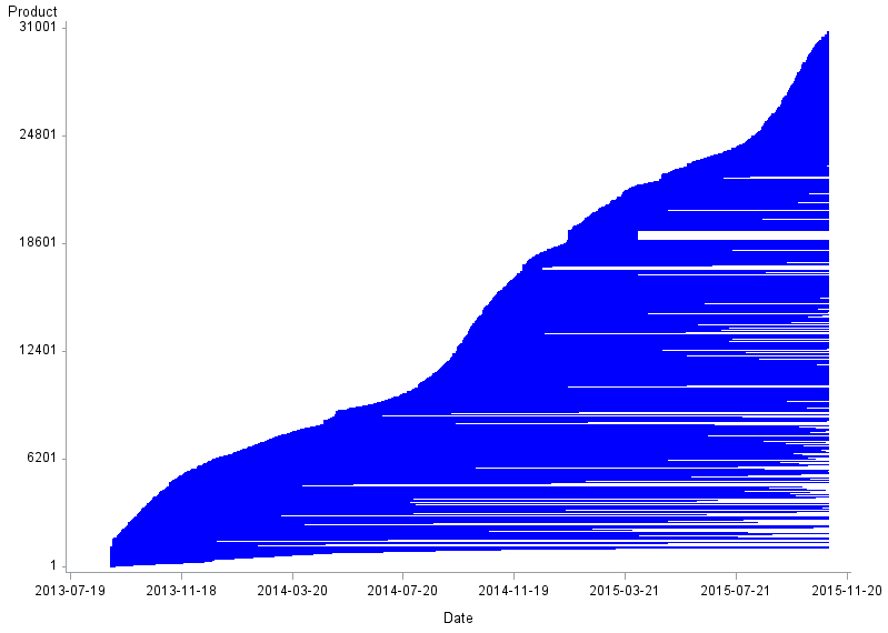
Source: Office for National Statistics, World’s Global Style Network
Download this image Figure 3: Churn for women's coats
.png (12.1 kB) .csv (881.6 kB)As with men's socks, we see reasonably high levels of product churn for women's coats (Figure 3). In this chart, however, the rate at which new products come into stock seems to vary over time. This manifests as a series of “humps” in the chart. These appear to occur every autumn, as the weather gets colder, corresponding to an increase in seasonal stock lines.
Figure 4: Product churn by item
UK, men’s clothing: August 2014 to October 2015; women’s clothing: September 2013 to October 2015
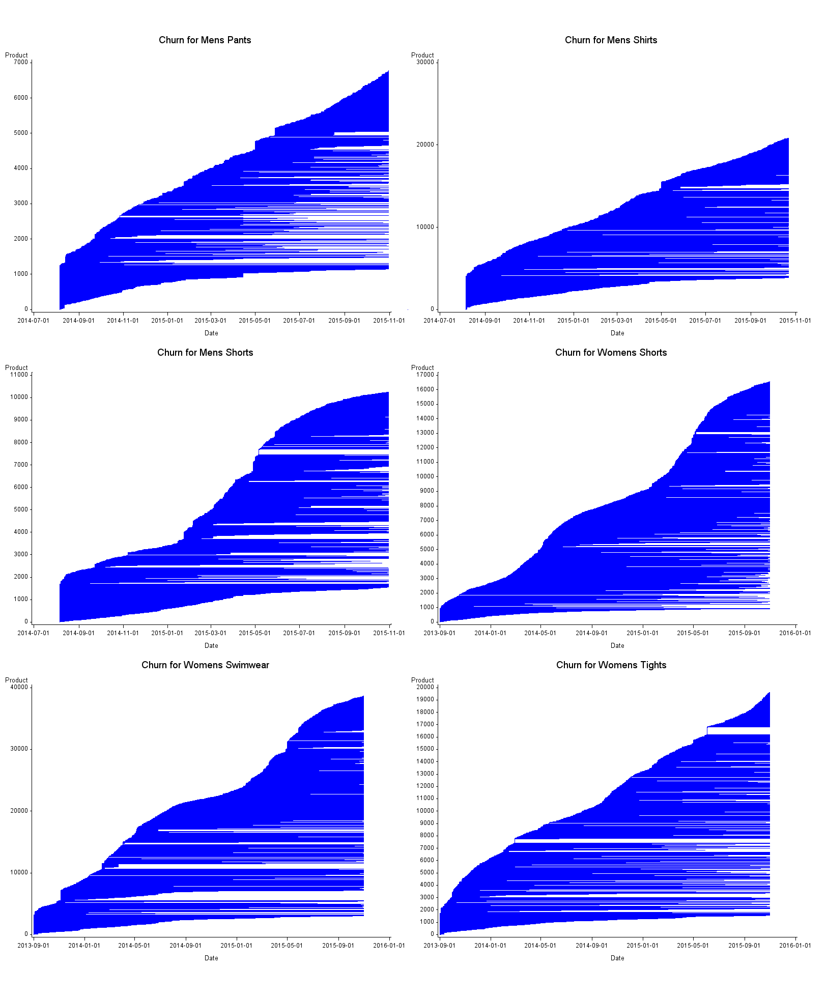
Source: Office for National Statistics, World’s Global Style Network
Download this image Figure 4: Product churn by item
.png (78.2 kB) .csv (3.0 MB)Churn plots for the remaining six clothing items are displayed in Figure 4. We see similar characteristics to those described previously in all of the plots. Men's shorts, and women's shorts and swimwear display some seasonality in the rate at which new products enter the dataset. There seems to be quite high levels of churn in most of the datasets. Also, all the plots seem to display some very short lived lines, to varying degrees.
Table 6: Products that do not churn
| Products with no churn | |||
| Item | Total number of products | Count | Proportion |
| Men's jeans | 14,667 | 4,997 | 34.07% |
| Men's pants | 6,781 | 1,880 | 27.72% |
| Men's shirts | 21,193 | 4,936 | 23.29% |
| Men's shorts | 10,250 | 2,423 | 23.64% |
| Men's socks | 9,665 | 2,563 | 26.52% |
| Women's coats | 49,241 | 7,421 | 15.07% |
| Women's shorts | 16,556 | 3,353 | 20.25% |
| Women's swimwear | 38,637 | 8,348 | 21.61% |
| Women's tights | 19,628 | 3,234 | 16.48% |
| Source: Office for National Statistics | |||
Download this table Table 6: Products that do not churn
.xls (18.4 kB)Table 6 gives the number and proportion of products that have not churned by the end of the time series. This is highest for men's jeans at 34.07% (that is, 4,997 product lines) and lowest for women's coats (15.07%) and women's tights (16.48%). This is in keeping with what has been observed in the churn plots.
Figure 5: Product churn for women's coats by retailer
UK, September 2013 to October 2015

Source: Office for National Statistics, World’s Global Style Network
Download this image Figure 5: Product churn for women's coats by retailer
.png (201.3 kB) .csv (1.8 MB)Figure 5 shows churn plots for women's coats for a selection of retailers. From the plots we can see that the churn behaviour varies very much from store to store. The number of women's coats on sale also varies from around 100 lines in, say, high street retailer L, to thousands in online retailer B.
The first behaviour pattern observed is where the churn plot is dominated by many long staying items. A typical example of this, again, is online retailer B. It seems likely that, whereas a high street retailer will need to refresh their stock, clearing out old lines to make space for new products, online fashion retailers will not necessarily have the same imperative to clear old stock, given the limitless space afforded them online.
The second pattern is for an almost complete periodic replacement of products. A typical example of this is high street retailer H, where there appear to be as many as five stock replacements within the time series. There remain some long staying items, but the overall trend is for the churn plot to show “blocks” of products. The blocks end each winter and summer, coinciding neatly with New Year and summer sales. It is also possible that unsold sales stock is transferred to specialist clearance stores, rather than put online.
The final pattern observed is where the churn appears to be rather more fluid. New lines are introduced gradually over the season and products churn both slowly and quickly. This is typified by a mix of both long and short tails in the plot. A good example of this is supermarket A; supermarkets, perhaps, having a broader appeal.
Table 7: Categorisation of retailer churn for women's coats
| Long staying | Fluid | Complete replacement | |
| Department store | A,E-F | D | B-C,G-H |
| High street retailer | F,L,N | A-C,E,J-K,M | D,G-I,P-R |
| Online retailer | A-C | - | - |
| Shoe specialist | - | C | - |
| Sports specialist | B | - | - |
| Supermarket | - | A-B | - |
| Source: Office for National Statistics | |||
Download this table Table 7: Categorisation of retailer churn for women's coats
.xls (17.9 kB)In Table 7, all retailers have been assigned to one of the three categories: long staying, complete replacement, and fluid. This is not a perfect categorisation as, in many instances, retailers exhibit behaviours that are typical of more than one category.
For instance, high street retailers I and R show some of the long and short tail churn typical of fluid behaviour; however, there is also evidence of some blocking, typical of complete replacement. In such cases, the categorisation has been selected that seems to best describe the underlying behaviour.
In other retailers, such as high street retailer L, there are too few products. A decision has been made on the basis of what data there is. In the case of high street retailer L, there does appear to be a complete replacement, but this is so slow that it is classed as long staying. Indeed, the entire long staying category might be composed of stores with very slow complete replacement.
The long staying category contains mainly online-only retailers (indeed, all three online retailers in the sample are included) and department stores (A, E and F). As discussed previously, this is an intuitive category for online stores to fall into. It may be that, as the big department stores are often supported by a website that allows them to expand their selection, they adopt a similar strategy to online-only retailers for their websites. The complete replacement category seems to contain mainly department stores and high street retailers. The fluid category is mainly comprised of high street retailers and both of the supermarkets in the sample are represented in this category.
It is also worth noting that internet-only stores tend to have many more products than other types of retailers, due to the limitless space available on a website. Online retailer B has slightly in excess of 5,000 lines for women's coats and, in fact, the department stores in the long staying category also carry many products; for example, department store A has just over 3,500 lines for women's coats. By contrast, the number of lines carried by smaller high street retailers doesn't exceed more than 1,500 lines for women's coats and is, on the whole, much fewer. A consequence of this is that the aggregated churn plots at item level are dominated by the long staying profile.
Proportional hazards regression
Explanation of the technique
In this section, we utilise a technique from survival analysis to better understand the churn in the data. Cox regression (also known as proportional hazards regression) is a regression technique, whereby a set of covariates is used to predict a survival function. This is a valuable technique as it uses both products that have and have not churned in the model estimation. In survival analysis, this would be patients who have and have not survived to the end of the trial. With web scraped data we can look at products whose lifecycle has ended and those which have not.
The procedure is based on two important assumptions:
a) observations are independent of one another
b) the hazard ratio is constant over time; this is known as the proportional hazards assumption
The following model equation gives us the hazard rate, hi(t) for product i at time t:
Equation 1
In this equation, Xik is the value of the kth covariate for product i and βk is the value of the estimated coefficient for covariate k. The hazard rate gives the potential for a product to churn at time t, given that it has not already churned up to time t. Larger values indicate a greater hazard. Note that this is a hazard rate, rather than a probability.
h0(t) is the baseline hazard rate at time t, which is independent of any of the covariates. The magnitude by which hi(t) differs from the baseline hazard rate is determined by the covariate values and estimated coefficients. Note that the model coefficients are constant over time. This gives rise to the proportional hazards assumption.
From the hazard function, we can deduce the survival function, Si(t), which gives the probability that product i will not have churned by time t. The survival function is the baseline hazard rate multiplied by the exponent of the integral of the hazard function over time. The survival function has a more intuitive interpretation than the hazard rate.
Data
The web scraped data does not include much additional information that we could use to construct covariates. It is reasonable to expect, however, that price behaviour could be used to predict time to churn. The price variable is used to construct the following variables:
- price change: this is the number of price changes that have occurred during the lifecycle of a product
- price relative: this is the price of a product at the end of its lifecycle relative to the price of the product at the beginning of its lifecycle – in other words, this is the price change over the lifespan
- final price: this is the final selling price of a product at the point of churn
- log final price: this is the natural logarithm of final price
- price band: dummy variables are created to indicate whether the starting price of a product is in a low, low-mid, high-mid or high price range – this is based on the 25th, 50th, 75th and 100th percentiles
In addition, the retailer information is used to create the following stratification variables:
- retailer: dummy variables are created for each of the retailers in the dataset
- churn type: dummy variables are created for the long staying, fluid and complete replacement churn categories, as defined in section 5.11. Note that the categories vary between items, so that the same retailer may display several different churn types.
In the analysis that follows we present results for women's coats only. The analytical process is very similar for all clothing items and it would be tedious to reproduce them in detail here. Women's coats has been selected as it has many of the characteristics of the other items: strong seasonality and a large number of records. It is also fairly typical of a high-churn fashion item; more so than, say, socks or pants. At the end of this section we compare the results for women's coats with the results for other clothing items.
Interpretation
Table 8: Hazards for women's coats UK, September 2013 to October 2015
| Variable | Parameter estimate | P | Hazard ratio | 95% confidence limits (Wald) |
| Price change | -0.127 | < 0.0001 | 0.881 | (0.875, 0.885) |
| Log final price | -0.161 | < 0.0001 | 0.851 | (0.824, 0.879) |
| Price relative | 0.6501 | < 0.0001 | 1.916 | (1.736, 2.114) |
| Low price | 0.8377 | < 0.0001 | 2.311 | (2.097, 2.546) |
| Low-mid price | 0.3365 | < 0.0001 | 1.4 | (1.329, 1.475) |
| Fluid | 0.1966 | < 0.0001 | 1.221 | (1.119, 1.332) |
| Department store A | 1.1446 | < 0.0001 | 3.141 | (2.916, 3.384) |
| Department store B | 1.3764 | < 0.0001 | 3.961 | (3.489, 4.497) |
| Department store C | 1.1899 | < 0.0001 | 3.287 | (2.847, 3.794) |
| Department store D | 2.6022 | < 0.0001 | 13.494 | (12.123, 15.020) |
| Department store E | 1.3468 | < 0.0001 | 3.845 | (3.598, 4.110) |
| Department store F | 0.8092 | < 0.0001 | 2.246 | (2.088, 2.416) |
| Department store G | 2.407 | < 0.0001 | 11.1 | (9.738, 12.653) |
| High street retailer E | 0.8121 | < 0.0001 | 2.253 | (1.982, 2.561) |
| High street retailer H | 1.2329 | < 0.0001 | 3.431 | (3.082, 3.820) |
| High street retailer I | 1.3838 | < 0.0001 | 3.99 | (2.850, 5.587) |
| High street retailer J | 0.6675 | < 0.0001 | 1.949 | (1.652, 2.300) |
| High street retailer M | 1.4107 | < 0.0001 | 4.099 | (3.665, 4.584) |
| High street retailer R | 1.5653 | < 0.0001 | 4.784 | (4.246, 5.390) |
| Online retailer B | -0.2117 | < 0.0001 | 0.809 | (0.755, 0.867) |
| Sports specialist B | 1.3791 | < 0.0001 | 3.971 | (3.338, 4.724) |
| Supermarket B | 0.7583 | < 0.0001 | 2.135 | (1.799, 2.534) |
| Source: Office for National Statistics | ||||
| Notes: | ||||
| 1. The reference category is price band: high or high-mid; churn: complete replacement, long staying; retailer: department store H; high street retailer A-D, F-G, K-L, N, P-Q; online retailer A, C; shoe specialist C; sports specialist A; supermarket A. | ||||
Download this table Table 8: Hazards for women's coats UK, September 2013 to October 2015
.xls (31.2 kB)The model coefficients for women's coats are presented in Table 8 and from the model we can identify the hazard ratio for each covariate. So, for example, the hazard of a women's coat churning in the low-mid price band is 40% greater than that of a product in the high or high-mid price band (which is the reference category), other variables remaining fixed. The churn hazard decreases as the price band increases, but is always greater than the churn hazard for the high price band. This suggests that the higher the starting price, the less a product's potential for churn.
Conversely, the churn hazard reduces by 12%, for each additional price change, all other variables remaining fixed. The churn hazard increases by 91.6%, for each unit increase in the final price relative to the start price, other variables remaining fixed. These results are counter intuitive. This suggests that prices are not reduced to clear old products. It may be that products with a longer lifespan have a greater incidence of price changes. It could also be that price reductions are the result of products coming on and off sale, rather than reductions to clear (which would also support the result for the number of price changes). The churn hazard decreases by 14.9% for each additional unit increase in the log of the final selling price, which sounds a more sensible result.
Counter-intuitive coefficients such as this could be evidence of multi-collinearity in the model, which is often a problem in hedonic regression. As a simple test, a model is constructed using only the erroneous variable as a covariate. In this model the sign of the coefficient remains in the counter-intuitive direction; a puzzling result.
Table 9: Hazard ratios for women’s clothing items UK, September 2013 to October 2015
| Hazard ratio | ||||
| Variable | Women's coats | Women's shorts | Women's swimwear | Women's tights |
| Price change | 0.881 | 0.857 | 0.885 | 0.888 |
| Final price | - | - | 1.001 | - |
| Log final price | 0.851 | - | - | - |
| Price relative | 1.916 | 2.032 | 2.01 | 0.785 |
| Low price | 2.311 | 1.373 | 0.832 | - |
| Low-mid price | 1.4 | 1.069 | 0.812 | 0.889 |
| High-mid price | - | - | 0.845 | 0.945 |
| Long staying | - | - | - | - |
| fluid | 1.221 | - | - | - |
| Department store A | 3.141 | 2.468 | 3.465 | 1.111 |
| Department store B | 3.961 | 2.441 | 1.601 | - |
| Department store C | 3.287 | 2.05 | 1.521 | - |
| Department store D | 13.494 | 10.772 | 11.5 | 3.194 |
| Department store E | 3.845 | 3.515 | 2.606 | 2.105 |
| Department store F | 2.246 | 2.032 | 1.794 | 1.304 |
| Department store G | 11.1 | 7.278 | 3.167 | 2.724 |
| Department store H | - | 3.942 | - | - |
| High street retailer A | - | 0.743 | 0.736 | 1.98 |
| High street retailer B | - | - | 8.238 | - |
| High street retailer C | - | 2.279 | 8.615 | 4.465 |
| High street retailer D | - | 3.264 | - | - |
| High street retailer E | 2.253 | 11.321 | 2.649 | - |
| High street retailer F | - | 1.522 | 1.233 | |
| High street retailer G | - | 3.928 | 7.666 | - |
| High street retailer H | 3.431 | 1.668 | 1.927 | 1.463 |
| High street retailer I | 3.99 | 2.09 | 2.806 | - |
| High street retailer J | 1.949 | 2.043 | - | - |
| High street retailer K | - | - | 1.425 | - |
| High street retailer L | - | - | - | - |
| High street retailer M | 4.099 | 2.634 | 2.955 | 2.446 |
| High street retailer N | - | - | - | - |
| High street retailer P | - | 4.708 | - | 1.87 |
| High street retailer Q | - | - | - | - |
| High street retailer R | 4.784 | 6.202 | 5.957 | 5.772 |
| Online retailer A | - | 1.324 | 1.69 | 2.601 |
| Online retailer B | 0.809 | 0.742 | - | 1.51 |
| Online retailer C | - | - | - | - |
| Shoe specialist A | - | - | - | - |
| Shoe specialist C | - | - | - | - |
| Shoe specialist D | - | - | - | - |
| Shoe specialist E | - | - | - | - |
| Sports specialist A | - | - | - | - |
| Sports specialist B | 3.971 | - | 0.679 | 1.301 |
| Supermarket A | - | 1.92 | 1.999 | 1.176 |
| Supermarket B | 2.135 | 2.448 | 2.161 | 1.55 |
| Source: Office for National Statistics | ||||
Download this table Table 9: Hazard ratios for women’s clothing items UK, September 2013 to October 2015
.xls (30.7 kB)
Table 10: Hazard ratios for men’s clothing items
| Hazard ratio | |||||
| Variable | Men's jeans | Men's shirts | Men's shorts | Men's pants | Men's socks |
| Price change | 0.876 | 0.864 | 0.79 | 0.833 | 0.85 |
| Final price | - | - | - | 1.015 | - |
| Log final price | 0.756 | 0.898 | 0.785 | - | - |
| Price relative | - | 1.551 | 2.314 | 0.434 | 0.53 |
| Low price | - | - | - | 1.961 | 0.763 |
| Low-mid price | 0.887 | - | 0.813 | 1.413 | 0.546 |
| High-mid price | - | - | 0.846 | 1.328 | 0.571 |
| Long staying | 0.916 | 0.372 | - | - | - |
| fluid | - | - | - | - | - |
| Department store A | 1.396 | 1.538 | 1.308 | 1.483 | - |
| Department store B | 2.278 | 0.705 | 1.455 | - | - |
| Department store C | - | - | 2.064 | - | - |
| Department store D | 2.903 | 1.819 | 10.049 | 2.302 | 2.08 |
| Department store E | 2.02 | 0.805 | 1.741 | 1.511 | 0.671 |
| Department store F | - | - | 0.822 | - | 0.724 |
| Department store G | - | - | - | - | - |
| Department store H | - | - | 5.193 | - | 0.748 |
| High street retailer A | 0.625 | 0.551 | 0.506 | - | - |
| High street retailer B | - | - | - | - | - |
| High street retailer C | - | - | 11.365 | - | 1.827 |
| High street retailer D | - | - | - | - | - |
| High street retailer E | - | - | - | - | - |
| High street retailer F | 0.604 | 0.4 | - | - | - |
| High street retailer G | - | 1.766 | 5.244 | - | - |
| High street retailer H | - | 0.448 | - | 0.582 | 0.507 |
| High street retailer I | - | - | 3.613 | 0.512 | 0.843 |
| High street retailer J | - | - | - | - | - |
| High street retailer K | - | 0.735 | - | - | - |
| High street retailer L | - | - | - | - | - |
| High street retailer M | - | 0.773 | 1.883 | - | 0.86 |
| High street retailer N | - | - | - | - | - |
| High street retailer P | - | 0.535 | - | - | 0.645 |
| High street retailer Q | - | - | - | - | - |
| High street retailer R | - | - | - | - | - |
| Online Retailer A | - | - | - | - | 2.735 |
| Online retailer B | 0.599 | 1.8 | 0.668 | - | - |
| Online retailer C | - | - | - | - | - |
| Shoe specialist A | - | - | - | - | - |
| Shoe specialist C | - | - | - | - | - |
| Shoe specialist D | - | - | - | - | - |
| Shoe specialist E | - | - | - | - | - |
| Sports specialist A | - | - | 0.473 | - | - |
| Sports specialist B | - | 3.848 | - | 0.355 | 0.417 |
| Supermarket A | 0.752 | 0.835 | - | 0.586 | - |
| Supermarket B | - | - | - | - | - |
| Source: Office for National Statistics | |||||
Download this table Table 10: Hazard ratios for men’s clothing items
.xls (31.7 kB)A similar procedure is used to produce a proportional hazards regression model for each clothing item. The hazard ratios for each respective item are provided in Tables 9 and 10. Note that the reference category for “retailer” is all retailers in the dataset (Table 1), but not included in the model. This is distinct from all retailers in the population, since we do not have data for all retailers. Moreover, the reference categories will, of course, be different for each clothing item, due to varying significance levels. Similarly, the reference categories for price band and churn will be those not included in the model (that is, those with no hazard ratios).
The variables for price change and department stores D and E are the only ones that are significant in all nine models. Price relative and department store A are significant in all but one model (men's jeans and men's socks respectively). The significance of department stores across all models is an intuitive result, as we would expect such stores to carry a wider breadth of stock.
Conversely, high street retailers L, N and Q, online retailer C, and shoe specialists A, D and E are not significant in any of the models. Some retailers specialise in women's (or men's) clothes and so are not significant in the models for men's (or women's) clothing. Department stores F and G, high street retailers H, M and R, and supermarket B are significant for all women's clothing models (although some also sell men's clothes). There are no retailers that are significant for all men's items and, on the whole, men's clothing items have fewer significant variables.
The hazard ratios are, in general, in the same direction and of a similar magnitude for all clothing items; for example, the hazard ratio for price change is generally between 0.850 and 0.888 for all clothing items, with one lower value at 0.790 (men's shorts). Of course, this is not always the case. Price relative hazard ratios for women's coats, shorts and swimwear, and men's shirts and shorts are all greater than one, whereas the hazard ratios for women's tights, and men's pants and socks, are all less than one. This suggests that the potential to churn for outer garments increases with the end price relative to the start price.
Conversely, for underwear, the potential to churn reduces as the price relative increases. If indeed regular sales do account for the increased churn hazard, this would imply that underwear does not go on sale as much as outer garments. This certainly seems reasonable. The hazard ratio for department store D is often high (greater than 10), suggesting that their products have a particularly large potential to churn. The churn plot for women's coats from department store D did show many short lived products.
The churn dummy variables are rarely significant. This may be because the categories are poorly defined: often retailers display overlapping churn behaviour and categorisations are based on a subjective judgement. It may also be that the retailer dummy variables are a better predictor, being at a more detailed level.
Figure 6: Survival plot for clothing items
UK, men’s clothing: August 2014 to October 2015; women’s clothing: September 2013 to October 2015

Source: Office for National Statistics, World’s Global Style Network
Download this image Figure 6: Survival plot for clothing items
.png (29.4 kB)Figure 6 shows the survival curve defined by the respective models for each of the nine clothing items. The survival curve usually depicts the baseline survival function for the given model. Since we have a different set of variables in the baseline for each item, we instead define the survival curve for a particular combination of variables that is common to all items.
We choose a “retailer” that is significant in all models. Churn type is derived from the choice of retailer. We use the median number of price changes and the mean price relative for all items. We assume that the starting price is the median price. Therefore our product is in the low-mid price band and the final price will be the median multiplied by price relative. So, each survival curve represents an item purchased from department store E, with a low-mid starting price (that is, the median), one price change and the final price is 20.99% lower than the starting price. Note also that the survival curves for men's clothing are shorter than those for women's clothing, due to the shorter time series.
We see that, for most items, the probability of surviving past 1 year is less than 0.1, with most being certain to churn at 2 years. The one exception is men's socks, where the survival curve is much more gradual than for other items. This suggests that men's socks are more long staying than other items and this certainly seems sensible.
Women's swimwear is the next shallowest curve which is, perhaps, a surprising result. Women's tights initially falls more steeply than women's swimwear; however, at just under 300 days, the curve flattens out and crosses the curve for women's swimwear. This suggests that, whilst initially women's swimwear products have a greater probability of not churning than women's tights, once they have been in the sample for 300 days, women's tights then have a greater probability of surviving. Perhaps there are two types of tights: more fashionable products that churn relatively quickly and classical styles that tend to remain in stock for longer periods of time.
The survival curve for men's jeans follows a similar path to women's swimwear, although the probability of surviving is less. Men's jeans still show a greater survival probability than many other items and this was certainly reflected in the churn plots. Men's shorts and shirts, for example, have very similar survival curves, both of which suggest a smaller probability of surviving compared to men's jeans.
Women's shorts and men's pants have smaller probabilities still and, in fact, up to about 150 days, men's pants have the lowest survival probabilities: an odd result. The survival curve for women's coats, finally, has by far the steepest descent and the sharpest elbow (the point at which the curve levels out). In the first few days, women's coats have the highest probability of surviving. By 200 days they have the lowest probability of surviving.
5.2 Analysis of price indices
Construction of indices
In this section we consider the construction of monthly price indices from web scraped data. Various different methods for compiling price indices are described in detail in the Appendix. Most of these methods were developed for use with scanner data.
Previous Office for National Statistics (ONS) research has looked at using some of these methods to produce web scraped price indices for grocery items (Breton et al., 2015; Breton et al., 2016). In this section we consider these methods applied to web scraped clothing data. Since we do not have expenditure data we cannot use the Törnqvist index as an input price index. In the Consumer Prices Index (CPI) and other international consumer price indices, the Jevons index is used to formulate item level price indices where no weights data are available. Therefore, we use the Jevons index as an input.
We attempt three different methods of compilation. First, a monthly chained index is constructed. As described in Appendix 2, this is typically avoided when constructing indices from scanner data, due to chain drift. However, this will not be an issue in web scraped data, where there are no expenditure weights. This is the simplest method and is worth considering.
Second, we consider a Gini, Eltetö and Köves, and Szulc (GEKS) approach. As we do not have detailed characteristic information, we are unable to use the Imputation Törnqvist Rolling Year GEKS (ITRYGEKS) method. We will, therefore, use the most recent method, which is the Intersection GEKS (IntGEKS).
Finally, in the absence of characteristic information, the Fixed Effects with a Window Splice (FEWS) index can be used to quality adjust for new items entering the index. Therefore, this method will also be used. Note that in the absence of weights, Ordinary Least Squares regression is used to estimate the coefficients and the resulting index is equivalent to a quality adjusted Jevons. These methods are all described in Appendix A.
We use unit prices to form price relatives. A unit price is an aggregate measure of the price of a product, or group of products, over a period of time. A unit price is calculated by dividing the total expenditure for the product over the period, by the total quantity of that product purchased in the period. This can be calculated using the following equation:
Equation 2
In this formula, pit is the price p of product i at time t, qit is the quantity purchased q of product i at time t, and f is the period frequency. As we do not have quantity data, we assume that quantities for each product are constant over time, which is simply the average price. This is shown with the following formula:
Equation 3
As we are using the Jevons formula to form price indices, we use the geometric average of prices for consistency. Krsinich (2014) suggests that weekly unit prices will result in the most accurate index (monthly index numbers can then be derived from the weekly index). However, due to processing constraints, Krsinich runs the analysis on monthly unit prices. We adopt a similar approach in this article.
For the purpose of this analysis, a product is defined by a unique identification code within a particular store. Therefore, the same product available in two different stores would be classed as two separate products. This is because there are different service levels associated with different retailers.
Before we present the item level clothing indices, it is worth considering national estimates of the same items. These item indices aggregate together to form part of the clothing and footwear division in the Consumer Prices Index (CPI), the current headline measure of inflation. There are, of course, a number of differences between these indices that make direct comparisons inappropriate.
CPI clothing prices are collected in stores across the country by price collectors. The price collectors will choose an item that is representative of what consumers will buy and that is also expected to remain in stock so that its price can be tracked over time. In the web scraped data, however, all prices are collected from websites regardless of expenditure.
As described in Section 5.1, products come in and out of stock rapidly, making it difficult to track items over time. CPI items are collected on a particular day in a month whereas a web scraper can collect prices daily. Extensive validation and cleaning procedures are applied to CPI data, which are beyond the scope of this article.
Finally, as discussed in Section 3, there are separate issues involved in the current measurement of clothing prices. Nonetheless, the CPI item indices still give a useful indication of the kind of behaviour that we might expect to see in clothing prices.
Figure 7: CPI index for women's coats
UK, September 2013 to October 2015
Source: Office for National Statistics, World’s Global Style Network
Download this chart Figure 7: CPI index for women's coats
Image .csv .xlsFigure 7 presents the women's coats index. We see some seasonal behaviour, with price increases occurring in winter months and very strong price decreases in the summer, particularly July. The general level of the index appears to be relatively constant over time, although it is hard to tell with a time series of this length.
Figure 8: CPI indices for clothing items
UK, men’s clothing: August 2014 to October 2015; women’s clothing: September 2013 to October 2015

Source: Office for National Statistics, World’s Global Style Network
Download this image Figure 8: CPI indices for clothing items
.png (92.4 kB) .csv (2.0 kB)The remaining CPI item indices are displayed in Figure 8. Many of the series exhibit seasonal behaviour, such as men's jeans, shirts and shorts. Others do not; women's swimwear is a surprising example and women's shorts is a very volatile series.
By contrast, men's socks, men's pants and women’s tights are very flat. The general level of the series are relatively flat in most cases, with exceptions for men's jeans and the early part of women's swimwear, where prices appear to be falling over time.
In all cases, the range of index points is much less than in women's coats: men's shorts have the largest range, with index points between 100 and 114.77. At the other end of the scale we have men's socks, with index points between 98.05 and 100.4. Indeed, we would expect there to be less variation in underwear items such as pants, socks and tights.
Figure 9: Analytical price indices for women’s coats
UK, September 2013 to October 2015
Source: Office for National Statistics, World’s Global Style Network
Download this chart Figure 9: Analytical price indices for women’s coats
Image .csv .xlsThe Jevons, IntGEKS and FEWS indices all behave in a similar fashion, descending rapidly over the time span to 16.27, 25.23 and 22 index points respectively. All three indices are very similar until early 2014, at which point the chained Jevons begins to descend more rapidly than the other methodologies. The IntGEKS and FEWS indices remain relatively close together until December 2014, at which point the FEWS index descends more rapidly, although not as markedly as the chained Jevons.
These indices are clearly an implausible measure of clothing price inflation as faced by consumers. Even if clothing prices were falling over the period, it would be extremely unlikely to be on quite this scale. These results are rather different to the published CPI results (Figure 7), which shows some seasonal movements, with peaks in September or October (of up to 103.31 index points) and falls in January (with a low of 75.90 index points). The underlying trend appears to be relatively flat.
Figure 10: Analytical price indices for web scraped clothing items
UK, men’s clothing: August 2014 to October 2015; women’s clothing: September 2013 to October 2015

Source: Office for National Statistics, World’s Global Style Network
Download this image Figure 10: Analytical price indices for web scraped clothing items
.png (214.7 kB) .csv (6.5 kB)Considering the other item indices in Figure 10, we see a very similar story. The Jevons, IntGEKS and FEWS indices descend implausibly towards zero. This is more pronounced in some indices than others. For example, the IntGEKS and FEWS indices for men's jeans only drop to 66.98 and 67.13 index points respectively. This is still not a convincing result, of course, and it seems likely that, given a longer time series, the indices would continue to fall.
The chained Jevons index remains much lower than other methods to varying degrees. This is less pronounced in some series, such as men’s shirts, women’s shorts and women’s swimwear; however, these are the series for which the IntGEKS and FEWS indices descend most rapidly, which perhaps accounts for the reduced divergence.
Analysis of price relatives
Looking closely at the price relatives for the chained Jevons and IntGEKS indices for women's coats gives us a better understanding of the underlying price behaviour that is driving these results. We concentrate on women's coats in this section for the same reasons as in the proportional hazards regression and to be consistent with that analysis.
The chained Jevons index compares unit prices relative to the unit price in the previous month. The survival curve in Figure 8 gave the probability of a woman's coat surviving for 1 month as 0.88, which is fairly high (although, of course, not all products in the sample will be new). Over 65% of the price relatives in the index are from four retailers: department stores A (12.82%), E (13.54%) and F (20.32%), and online retailer B (21.16%). Department store E was used as the baseline retailer for the survival curve and, in our proportional hazards regression model (Tables 9 and 10), the hazard ratios for the other three retailers were lower than for department store E, suggesting that their products have even less potential to churn.
Moreover, we identified all of these retailers as showing long staying churn behaviour. Therefore, we can expect a reasonable representation of up-to-date lines in the index. All of these retailers show more decreases than price increases (department store A: 53.79% decreases and 30.56% increases; department store E: 53.99% decreases and 33.58% increases; department store F: 54.55% decreases and 28.57% increases; and online retailer B: 48.53% decreases and 27.97% increases;). Therefore, we look at the price relatives in more detail.
To begin, we decompose the Jevons formula into three components: a component where the price relatives are greater than one, a component where they are less than one, and a component where they equal one. This can be done using the following equation:
Equation 4
In this equation, n1 + n2 + n3 = n, which is the number of products, and p ̅tj, > p ̅0j, p ̅tk = p ̅0k and p ̅tl < p ̅0l. We can then cancel the k terms, as shown in the following equation:
Equation 5
Figure 11: Price relatives for women's coats
UK, September 2013 to October 2015
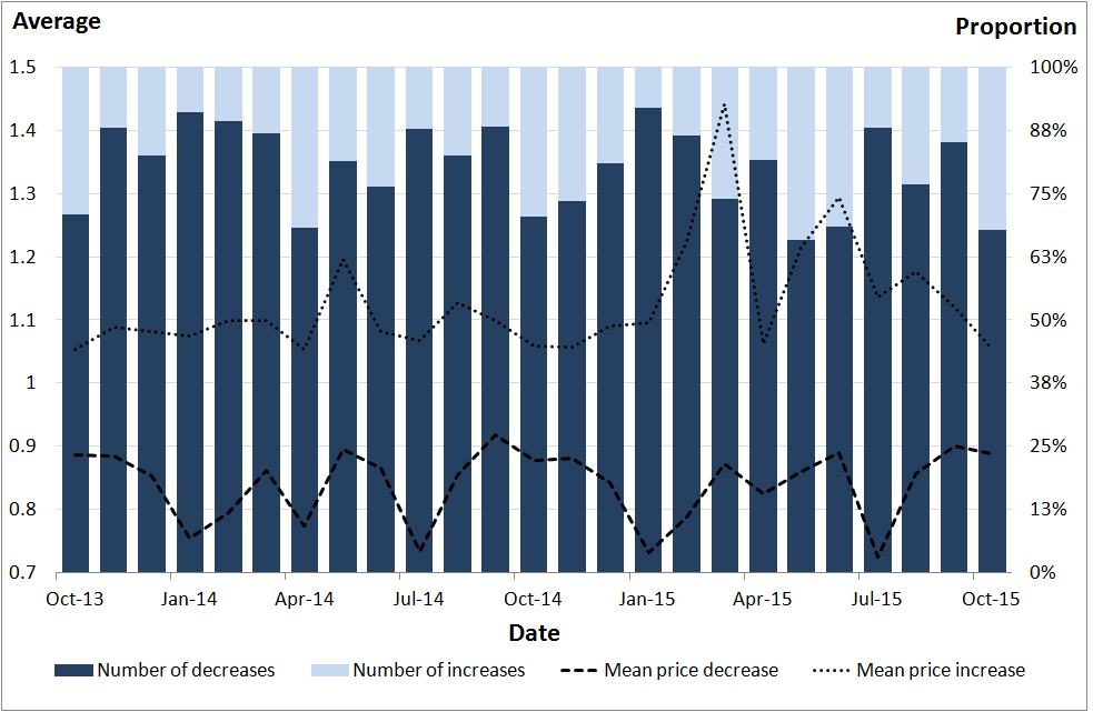
Source: Office for National Statistics, World’s Global Style Network
Download this image Figure 11: Price relatives for women's coats
.png (78.4 kB) .csv (1.1 kB)Figure 11 compares the number of price increases (n1) with the number of price decreases (n3). The bars show these as a proportion of the total number of price increases and decreases. The average price increase and decrease are also shown.
The average price decrease varies from month to month between roughly 0.7 and 0.9. The average price increase is more stable, at around 1.1, until early 2015 when we see movements of between roughly 1.1 and 1.4. If we disregard instances of no price change, the sample is dominated by price decreases. The proportion of price decreases varies between approximately 65% and 90%.
Figure 12: Price decreases and differenced chained Jevons index for women’s coats
UK, September 2013 to October 2015
Source: Office for National Statistics, World’s Global Style Network
Download this chart Figure 12: Price decreases and differenced chained Jevons index for women’s coats
Image .csv .xlsFigure 12 shows the number of price decreases each month. This is overlaid with the differenced chained Jevons series. Differencing the series (that is, subtracting the current value from the previous value) has the effect of removing the trend from a series or, in other words, making it stationary. This allows us to compare the movements in the index directly with the price decrease series, which is, by nature, stationary.
The number of price decreases appears to show some seasonal behavior, with more decreases month on month in the run up to Christmas and peaking in January. The number of price decreases then drops over the spring and summer months. This is partially intuitive: we would expect to see a large number of price decreases in January, coinciding with the January sales, and the post-January drop is consistent with the end of sales and introduction of new stock. However, the reason for the increasing number of price drops in pre-Christmas and winter months is perhaps less clear.
The peaks in the differenced chained Jevons series appear to coincide well with peaks in the price decrease counts. (It is worth noting that differencing has not removed the downward trend entirely; however, it does allow us to see where there are similar movements in the two series). This suggests that the movements in the series may be driven by how prevalent price decreasing strategies are. Nonetheless the dynamics of the series are dominated by the downward trend, which can only be driven by falling prices.
It is also important to remember that the act of chaining “magnifies” index movements somewhat since Pt-1,t and Pt,t+1 are greater than 1, then Pt-1,t × Pt,t+1 is greater than both Pt-1,t and Pt,t+1; and similarly, if Pt-1,t and Pt,t+1 are less than 1, then Pt-1,t × Pt,t+1 is less than both Pt-1,t and Pt,t+1.
We now consider the IntGEKS index. The price relatives in the IntGEKS index are dominated by the same four retailers: department stores A (14.20%), E (14.95%) and F (22.99%), and online retailer B (25.75%). Again, over the period, each retailer has a greater proportion of price decreases (department store A: 48.28% decreases and 38.34% increases; department store E: 51.46% decreases and 39.86% increases; department store F: 48.48% decreases and 40.68% increases; and online retailer B: 46.69% decreases and 38.24% increases).
We use a similar decomposition to analyse the price relatives. The structure is much more complex than the chained Jevons index, so we begin by considering the IntGEKS formula as the product of left and right-hand side arguments, using the following equations:
Equation 6
In this equation, PU0,T is the input price index P compiled from prices for products in the set U, with a base period 0 and current period T, and U0,T is the sample of products available in periods 0 and T.
Since the input price index is a Jevons index, we use the Jevons decomposition in Equation 5 to investigate the price relatives. Figure 13 gives the average and number of price increases, decreases and no changes for both the left- and right-hand sides of the IntGEKS equation. For the sake of simplicity, this is presented for the first 13-month window only.
Figure 13: Price relative decomposition in the IntGEKS equation
UK, men’s clothing: August 2014 to October 2015; women’s clothing: September 2013 to October 2015

Source: Office for National Statistics, World’s Global Style Network
Download this image Figure 13: Price relative decomposition in the IntGEKS equation
.png (159.9 kB) .csv (17.8 kB)The first point to note is that, when the link period t is equal to the base period T-1 then PT-1,t=1. Therefore, on the left-hand side charts, we see no price changes at this point in time. Similarly, when the link period t is equal to the current period T then Pt,T=1 and we see no price changes on the right-hand side charts.
Secondly, the number of price relatives decreases as the link period t moves further away from the base period T-1 on the left-hand side charts and from the current period T on the right-hand side charts. This is because the matched set of products i∈UT-1,t,T decreases the further t is from T-1 and T respectively. This is a sensible result, as it suggests that a product is more likely to be out of stock the further it is from the reference period.
Indeed, after 13 months, we would expect to see new stock replacing last year's products. The survival curve presented in Figure 6 (survival curve) gave the probability of a product surviving after 1 month as approximately 0.88, decreasing to 0.5 after 98 days. At 6 months, the probability of survival is 0.05, and after 13 months it is, in fact, virtually zero. Therefore, it is likely that any products left in the sample when the link period is 1 or 13 will be very near the end of their lifespan and are most likely experiencing heavy price reductions.
Because the IntGEKS index is a matched index, and because the sample will decrease as the link period moves away from the base and current periods, in distant link periods we will only detect price movements associated with old lines and will fail to detect the price movements of new products. Because of the level of churn in fashion items, this is likely to cause particular problems.
Finally, both the average price increase and the average price decrease appear relatively stable regardless of the link period. In Figure 14, in the left-hand side charts there is a slight drop in the average price increase just before the link period and in the average price decrease just after the link period. In the right-hand side charts there is typically a slight uplift in the average decrease just before the link period and in the average increase just after the link period. We will discuss this further in due course.
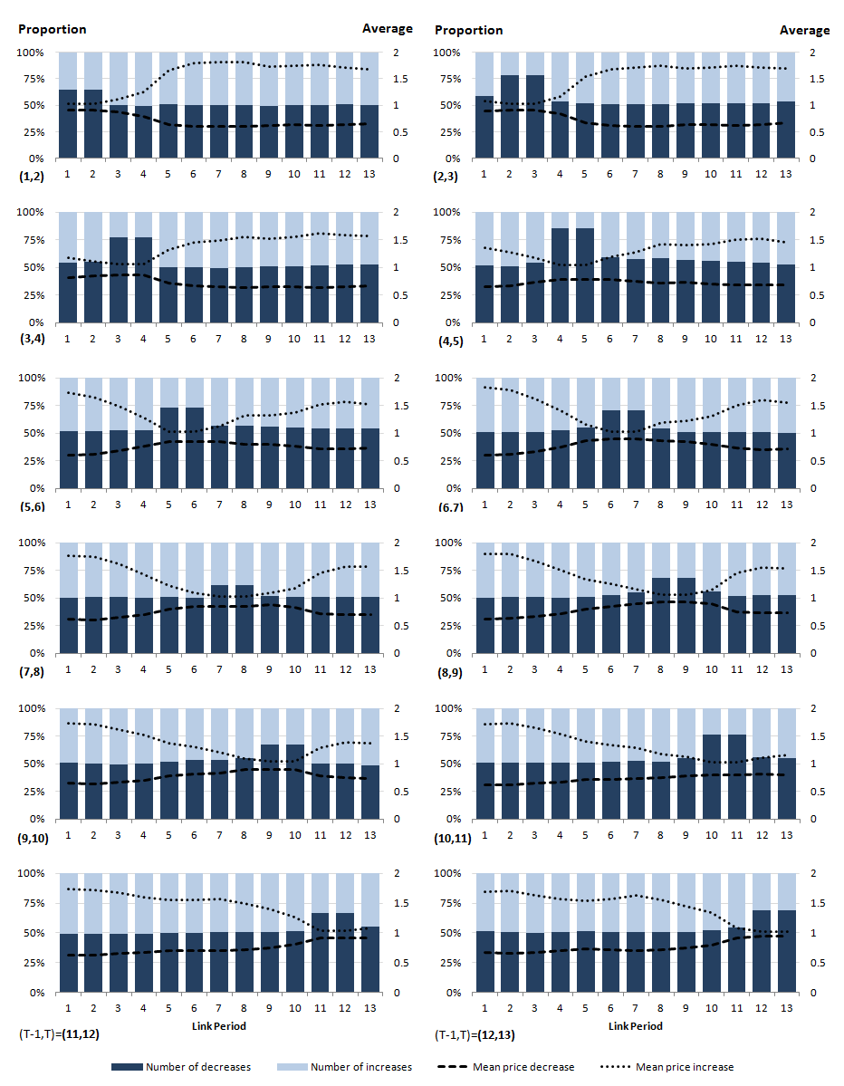
Figure 14: Proportional price relative decomposition in the IntGEKS equation
UK, men’s clothing: August 2014 to October 2015; women’s clothing: September 2013 to October 2015

Source: Office for National Statistics, World’s Global Style Network
Download this image Figure 14: Proportional price relative decomposition in the IntGEKS equation
.png (179.2 kB) .csv (19.7 kB)We next consider the number of price increases and decreases as a proportion of total price changes. Figure 14 highlights that, on the left-hand side, price decreases are much more frequent after the link period, whereas price increases are much more frequent before. After the link period we have T-1 < t. Price decreases suggest that pit / piT-1 < 1. This indicates that prices are falling, since the earlier price in the denominator is larger than the later price in the numerator. Before the link period we have T-1 > t. Price increases suggest that pit / piT-1 > 1. This indicates that the earlier price in the numerator is larger than the later price in the denominator. This also suggests falling prices.
On the right-hand side, we have the converse situation, with more price decreases before the link period and more price increases after the link period. After the link period T < t, so price increases indicate larger prices in the early period (piT / pit > 1). Similarly, before the link period, where T > t, we have price increases, indicating that earlier prices are greater than later prices (piT / pit < 1). Again, prices are falling.
We see similar behaviour in the average price increases and decreases. All the evidence in the graphs, therefore, suggests a picture of falling prices for women's coats, which is certainly what we see in the IntGEKS index. This supports our idea from Figure 13, that the length of the IntGEKS window means that prices from products very near the end of their lifecycle are being drawn into the calculation. These products are most likely accompanied by steep price reductions. But why is the downward trend in the index so extreme?
To answer this question we first note that, in each chart, where the link period is equal to the price reference period we, of course, have no price increases or decreases. When the left- and right-hand sides are multiplied together this will give more weight to the greater number of price decreases on either side in these periods. In other words, when T-1=t on the left-hand side, the corresponding t on the right-hand side is a decrease.
Similarly, when T=t on the right-hand side, the corresponding t on the left hand side is a decrease. In other periods, we are multiplying a greater number of increases (or decreases) on the left hand side, with a greater number of decreases (increases) on the right hand side. We might expect these to cancel out, given the relative flatness of average price increases and decreases. In fact, there are also mathematical reasons for this cancellation. As we are using the Jevons index as an input into the IntGEKS procedure, we have:
Equation 7
which is simply the average of (T+1) JevonsT-1,T indices, with slightly different samples (based on the matched set UT-1,t,T for each t∈{0,…,T} ). This occurs because the left and right hand sides of the equation are based on the same matched set, which would not be the case for, say, a standard GEKS-Jevons index. This result does seem to suggest that the IntGEKS-Jevons index is somewhat invalid, especially considering the complexity of the calculations involved. Of course, if a Törnqvist index is used, as recommended in the literature, there would be no issue, since:
Equation 8
and, in general, siT-1 ≠ siT (where sit is the expenditure share s for product i in period t). Therefore, the IntGEKS method is more appropriate when data on expenditure shares are available. Nevertheless, there remain marked differences between the IntGEKS results and the chained Jevons results. As a result of Equation 7 we can disregard the left-hand / right-hand side formulation and consider the aggregate price relatives in each link period. Figure 15 presents charts for these price relatives over the first thirteen months for women's coats.
Figure 15: Proportion of price relatives in the IntGEKS-Jevons equation
UK, men’s clothing: August 2014 to October 2015; women’s clothing: September 2013 to October 2015
Source: Office for National Statistics, World’s Global Style Network
Download this image Figure 15: Proportion of price relatives in the IntGEKS-Jevons equation
.png (96.7 kB) .csv (9.1 kB)Here we see that, in months where the link period is not equal to the base or current period, the number of price increases and decreases are roughly equal. In the 2 months where the link period is equal to either the base period or the current period, there are a greater number of price decreases. Note also that, in these two periods, the average price decrease is greater and the average price increase is less than in other periods. This is a direct result of the observations made on Figure 14. It is precisely this greater number of decreases that is contributing to the IntGEKS index's downward movement and once these decreases are compounded month-on-month, the decrease becomes terminal.
This is not necessarily a bad thing, as the IntGEKS index is doing what it should and identifying the falling of prices. The issues are pertinent to the measurement of price changes in clothing in general. Compilation methods that rely on matched products are problematic. These methods are based on the assumption that each product identifier represents a unique product in the eyes of the consumer. This definition is too tight. Therefore, the rapid churn associated with clothing products causes the index to fall.
For example, a coat that is available in December 2015 may not have the same value to a consumer in December 2016, as it may no longer be considered fashionable. A fashionable coat in 2015 could be replaced by a fashionable coat in 2016. This may not be the same product and there may be many products that could be a valid replacement. One solution might be to average over several products, where the quality is not considered to be significantly different.
The result in Equation 7 is a general result for the IntGEKS-Jevons index. The analysis of price relatives, however, was conducted specifically on the indices for women's coats, constructed from WGSN's web scraped data. As such, this set of results is particular to this analysis and does not generalise. Of course, in the case where other items exhibit the same underlying behaviours observed here, we could make the same observations; however, without further analysis of their price relatives, we cannot say that this is the case.
We do not attempt an analysis of the FEWS index in this article.
Notes for: Analysis
- Note that the categories vary between items, so that the same retailer may display several different churn types.
6. Conclusions
The web scraped clothing data analysed in this paper offer us the opportunity to improve our understanding of a difficult to measure area of consumer price indices. The rapidity with which clothing items come in and out of stock will cause issues for index number methods that rely on matching products over time.
Our analysis has shown different levels of churn for different items of clothing. For example, men's jeans tend to have quite a long lifespan, with new products coming into stock at a steady rate. Conversely, women's swimwear products churn much sooner and the rate at which new items come into stock depends on the season. We also see different retailers exhibiting different churn behaviours. Some seem to have a periodic near complete replacement of their stock, while others' products tended to be very long staying, with little churn.
Due to the large volume of products held by internet-only retailers, the long staying churn pattern tends to dominate churn behaviour at the all retailers level. In other retailers we see a more fluid pattern of churn, with both long and short staying products. The average lifespan of a product is just over a season (typically between 80 and 120 days) and, in a typical month, somewhere between 12% and 18% of products churn. Only between 0% and 6% of products are in stock for the entire duration of the index.
We used proportional hazards regression to calculate hazard ratios for each item. The number of price changes proves to be a good predictor of the churn hazard, with the potential to churn decreasing with the number of price changes for all items. Other universally significant predictors are retailer dummy variables for department stores D and E. The potential for a product from department store D to churn is always greater than the baseline and more than 10% greater in many cases. We derived survival probabilities for each of the nine clothing items. For most items, the probability of survival drops below 0.1 within the year.
We used the chained Jevons, IntGEKS and FEWS methods to construct price indices from the data. In all cases, the indices decline rapidly over the period. This was by as much as 80 or 90 index points for some of the women's clothing items (coats, shorts and swimwear), and the Jevons indices always decline fastest. This is clearly not a plausible indication of the price changes experienced by consumers. Analysis of the price relatives for women's coats suggests that a greater number of price decreases are driving the index's descent.
Analysing the churn in this data has helped to understand the driving factors behind the price index behaviour. There remains more work to be done, however, if a plausible price index for clothing items is to be constructed from the web scraped data. One approach would be to consider ways of averaging over similar products to create a looser product definition. We have recently developed a technique for clustering similar products, using these clusters to form a price index (Metcalfe et al, 2016). Future work will explore this technique with the WGSN data.
Back to table of contents7. References
Breton, R., Clews G., Metcalfe, L., Milliken, N., Payne, C., Winton, J. and Woods, A. (2015) Research indices using web scraped data.
Breton, R., Flower T., Mayhew M., Metcalfe, L., Milliken, N., Payne, C., Smith T., Winton, J. and Woods, A. (2016) Research indices using web scraped data: May 2016 update.
De Haan, J. (2015) Rolling year time dummy indexes and the choice of splicing method, paper presented at the 14th meeting of the Ottawa group, Tokyo, 20 to 22 May 2015.
De Haan, J. and Hendriks, R. (2013) Online data, fixed effects and the construction of high-frequency price indexes, paper presented at the 13th Economic Measurement Group, Sydney, 28 to 29 November 2013.
De Haan, J. and Krsinich, F. (2012) The treatment of unmatched items in rolling year GEKS price indexes: evidence from New Zealand scanner date.
De Haan, J. and van der Grient, H. (2009) Eliminating chain drift in price indexes based on scanner data, Journal of Econometrics 161 (1) pp 36 to 46.
Diewert, W.E., Fox K,J., and Ivancic, L. (2009) Scanner data, time aggregation and the construction of price indexes, Journal of Econometrics 161 (1) pp 24 to 35.
Greenlees, J.S. and McClelland, R. (2010) Superlative and regression-based consumer price indexes for apparel using U.S. scanner data, paper presented at the Conference of the International Association of Research in Income and Wealth, St. Gallen, 27 August 2010.
International Labour Organisation (2004) Consumer price index manual: theory and practice.
Krsinich, F. (2014) The FEWS index: Fixed effects with a window splice, paper presented at the Group of Experts on Consumer Price Indices, Geneva, 27 May 2014.
Krsinich, F. (2015) Price indexes from online data using the fixed-effects window-splice (FEWS) index, paper presented at the 14th meeting of the Ottawa group, Tokyo, 20 to 22 May 2015.
Krsinich, F. and Lamboray, C. (2015) A modification of the GEKS index when product turnover is high, paper presented at the 14th meeting of the Ottawa group, Tokyo, 20 to 22 May 2015.
Metcalfe, L., Flower T., Lewis T., Mayhew, M. and Rowland, E. (2016) Research indices using web scraped data: clustering large datasets into price indices (CLIP).
Nygaard, R. (2015) The use of online prices in the Norwegian consumer price index, paper presented at the 14th meeting of the Ottawa group, Tokyo, 20 to 22 May 2015.
Office for National Statistics (2011) CPI and RPI: increased impact of the formula effect in 2010.
Back to table of contents8. Appendix 1: Index number formulae
There are many different formulae for compiling a price index and, to some extent, the choice of formula will depend on the data available and the purpose of the index. In this section we will focus on two methods, which will be used as inputs into new methods: the Törnqvist index and the Jevons index.
The Törnqvist index is typically used in the literature when the methods are applied to scanner data. This is because it is a superlative index, which approximates the effect of consumer substitution. Consumers will substitute goods and services whose prices are increasing rapidly with goods and services whose prices are increasing less quickly. The Törnqvist index is also a symmetrical index, which means that the average of the expenditure shares from the current and base periods are used. There is an intuitive appeal to using expenditure information from both periods. The general form of the Törnqvist index can be calculated using the following equation:
Equation 9
In this equation pit is the price p of a product i at time t, and sit is the expenditure share s for product i at time t. Period 0 is the base period. This may be t-1, or it may be some fixed point in the past. There are n products in the sample.
Where expenditure information is not available, National Statistical Institutes (NSIs) will often use the Jevons formula to compile price indices. The Jevons formula arises from the stochastic, or statistical, approach to index numbers. It is assumed that random variations in the price relatives are multiplicative and will follow a lognormal distribution with a mean of zero. This gives rise to the following formula:
Equation 10
This is the geometric mean of price relatives. The Jevons formula is more useful when we are discussing web scraped data, as it does not require expenditure data.
One further formula used to compile indices where expenditure information is unavailable is the Carli equation:
Equation 11
This is used to calculate the arithmetic average of price relatives. This method has been shown to behave badly in certain circumstances and is not generally used in the compilation of price indices internationally1.
Appendix 1: Index number formulae
- One notable exception is the Retail Prices Index (RPI). RPI lost its National Statistics status in 2013 due to its use of the Carli formula.
9. Appendix 2: Chained bilateral index
In national consumer price indices a fixed base, or direct index, is typically used. This means that the same products are followed for the duration of the index1. This is sensible in traditional price collection as a comparable replacement can be identified to replace a product that is no longer stocked. Web scraped or scanner data, however, typically have a very high level of product turnover; that is, products coming in and out of stock. This makes the use of fixed base methods, which rely on matched data, problematic. The use of a fixed base period means that the number of matches will decrease over time, as the current product selection becomes less representative of the initial product selection. This reduces the sample size and means that new products will not be introduced into the index.
An intuitive approach to compiling price indices from larger datasets, therefore, is to use the previous period as the base period for each bilateral comparison. These can then be chained together to form a continuous index using the following formula:
Equation 12
In this formula P0,t is the price index between period 0 and period t. This is known as an indirect index, but is also often referred to as a daily, weekly or monthly chained bilateral index. Chaining at each time point allows the basket to be flexible, reflecting the products that are in the sample at each particular point in time.
Both direct and indirect approaches are investigated, using Laspeyres and Paasche index number formulae in the seminal paper by Diewert, Fox and Ivancic (2009). Diewert, Fox and Ivancic (2009) identified issues with chain drift when using indirect indices on scanner data. This is exacerbated by the use of frequent chaining. The International Labour Organisation (ILO) Consumer Prices Index manual defines chain drift as when an index that has been chained “does not return to unity when prices in the current period return to their levels in the base period” (ILO, 2004, p.445).
One phenomenon that is thought to exacerbate chain drift is when retailers put products on sale. Consumers will then “stock up” on products with a long lifespan, increasing expenditure. When prices return to pre-sale levels, expenditure on these items drops. Under traditional price collection methods, expenditure weights are not available at the product level, so the indices are unaffected by this phenomenon. Scanner data, however, contain detailed price and quantity information at the transaction level.
Notes for: Appendix 2: Chained bilateral index
- In the UK this is 13 months. Annual indices are then chained together to form a continuous time series.
10. Appendix 3: GEKS approach
Diewert, Fox and Ivancic's paper (2009) proposes using the Gini, Eltetö and Köves, and Szulc (GEKS) method – originally designed for purchasing power parities – to eliminate chain drift in price indices constructed from scanner data.
Purchasing power parities compare prices between countries rather than over time. They show the change in price of a fixed basket of goods and services in a particular country relative to an arbitrary base country. For example, if the base country were the UK, how much more would the basket cost if it were purchased in Germany, say, than the UK?
Chaining is often necessary in the production of official indices. It is not unreasonable to expect that the price change measured directly between two countries should be the same as if two indices were indirectly chain linked together. Using our example previously mentioned, we would expect that the direct index for Germany based in the UK should be the same as chain linking together the index for France, say, based in the UK, and the index for Germany based in France. The GEKS index, then, ensures this transitivity property by taking the geometric mean of all indirect indices.
Hence, the GEKS index will be free of chain drift, since:
Equation 13
Chaining the indices together does not result in the index “drifting” from the direct index. Another obvious advantage of the GEKS index is that it makes use of as much of the available data as possible through a flexible basket, as with monthly chained indices. The authors utilise the GEKS index by redefining it in the time domain using the following equation:
Equation 14
11. Appendix 4: RYGEKS
One drawback with using the GEKS index for temporal indices is that whenever a new time point is added, the entire index will be revised. In official statistics, consumer price indices are rarely revised. Of course, it would be quite possible to simply splice the latest movement in the GEKS index to the existing time series; however, the problem with this approach – and the reason that GEKS is generally not used to create temporal indices – is that, over time, this will lead to a loss of characteristicity.
Characteristicity is the extent to which an index is based on relevant data: for temporal indices a characteristic index should be based on recent data. Hence, the more time points that are added, the less characteristic the GEKS index will become. For this reason Diewert, Ivancic and Fox propose a Rolling Year (RY) GEKS approach (formalised in De Haan and van der Grient, 2009). A 13-month rolling window is recommended as this will allow "comparison of strongly seasonal items" (De Haan and van der Grient, 2009), whilst minimising the window length and, hence, loss of characteristicity.
Therefore, using a 13-month rolling window, the general form of the RYGEKS index is as follows:
Equation 15
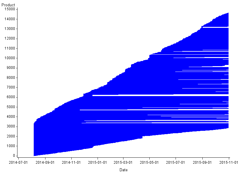
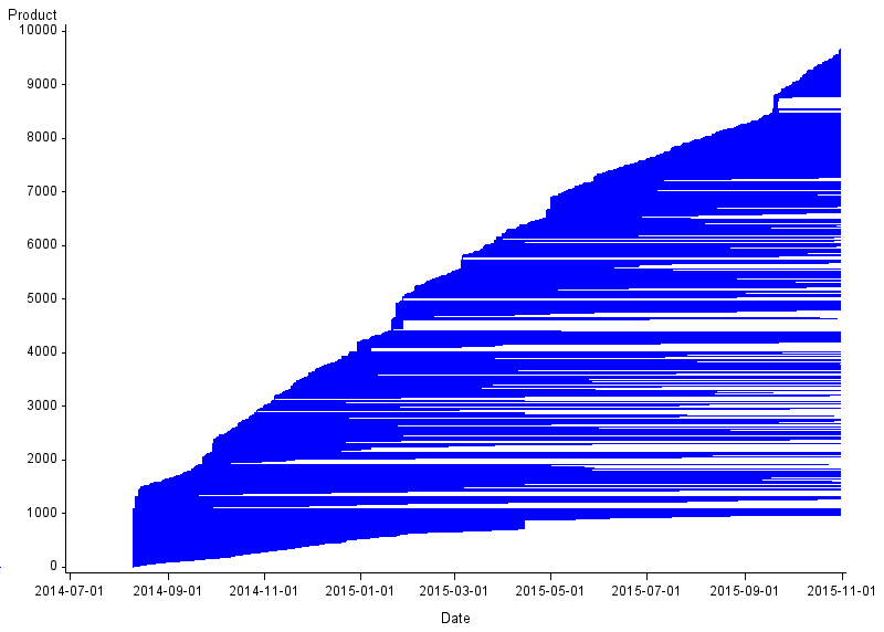
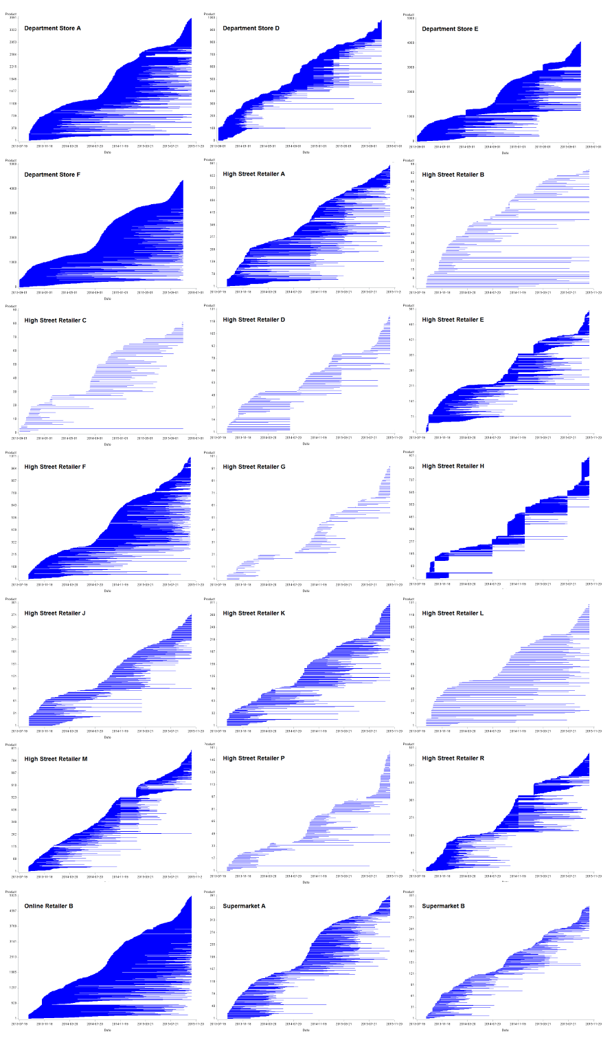
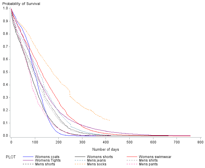
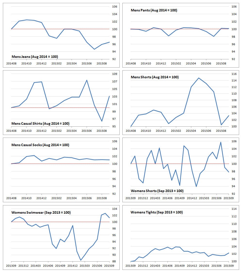
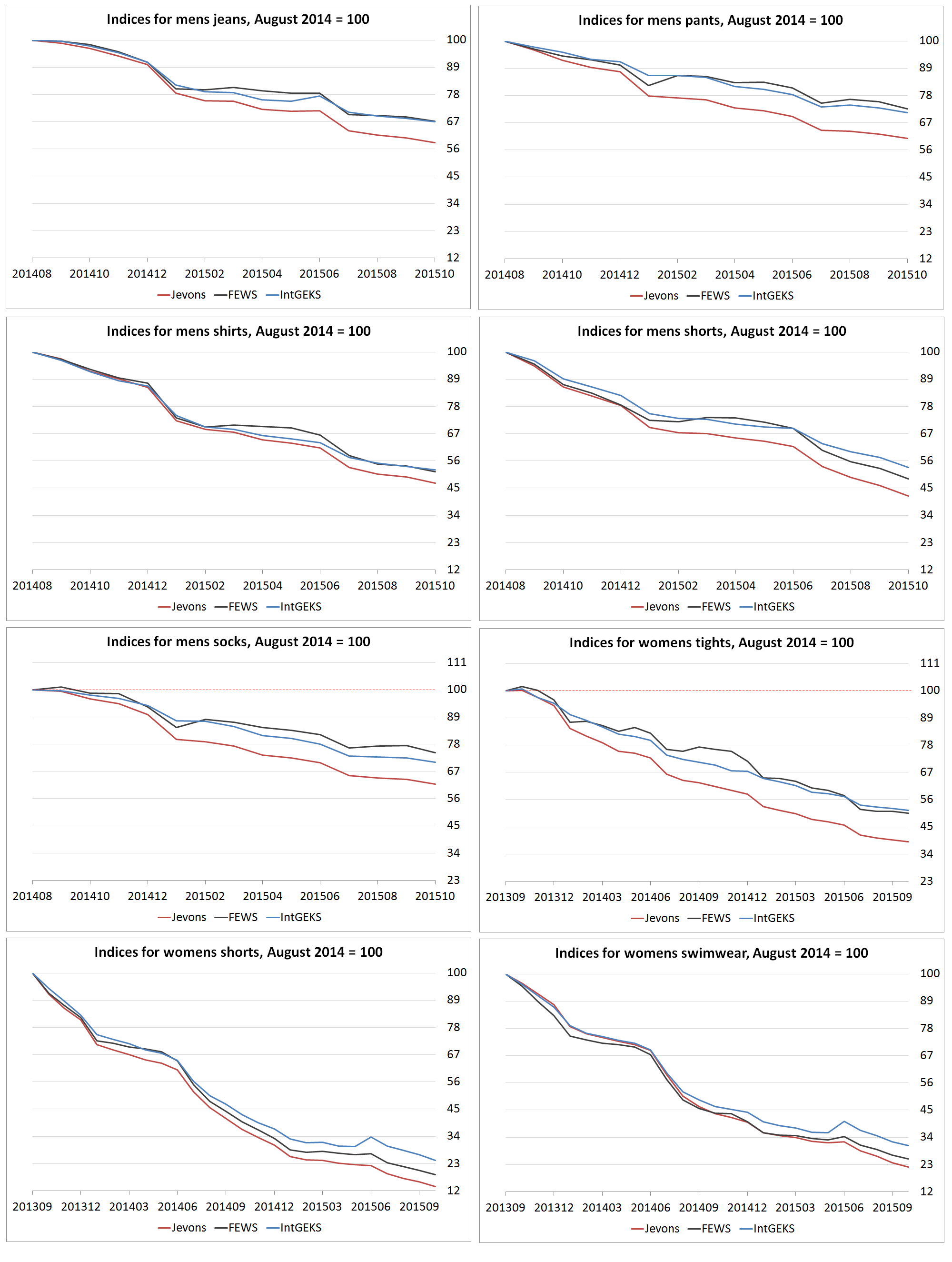
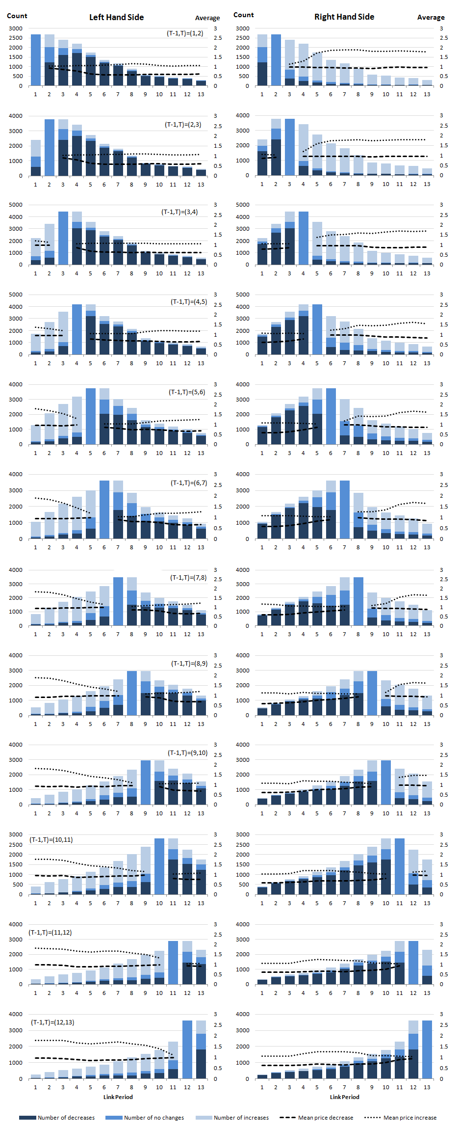
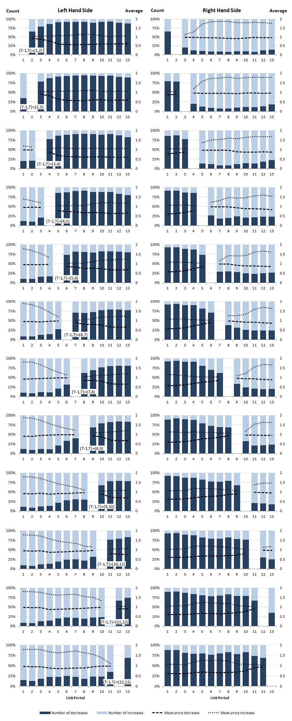
Using the rolling year method, however, means that the RYGEKS index is not transitive. The extent of the loss of transitivity, though, is thought to be negligible. We would, moreover, expect the RYGEKS index to be approximately free from chain drift. A major advantage of the GEKS, and indeed the RYGEKS, methods is that, through an increased number of matches, they make maximum use of available data. A further implication of this is that there is no need to impute missing prices.
Back to table of contents12. Appendix 5: ITRYGEKS
Whilst there is no need to impute missing prices using the RYGEKS method, it is still necessary to account for quality changes that are associated with the introduction of new products and the disappearance of old products. This is, perhaps, clearest in technological goods, where an improvement in a product's specification coincides with the release of a new model, potentially at a new price point. Therefore, there is an implicit price movement associated with the introduction of new goods that will not be captured using the standard RYGEKS method, but which it is particularly important to capture when consumers increasingly purchase goods of a higher quality.
To address this issue, De Haan and Krsinich (2012) propose an Imputation Törnqvist (IT) variant of the RYGEKS index. This uses hedonically adjusted Törnqvist indices as the input price index P0,t in a RYGEKS procedure. Hedonic regression assumes that the price of a product is uniquely determined by a set of K characteristics (for example, screen size, processing speed and storage would be characteristics for a laptop). Regression on the log of price is then used to estimate parameters for each of these characteristics, from which we can predict the price with quality held constant. This technique is typically used for technological items, where the pace of change is swift. In the UK's Consumer Prices Index (CPI), laptops, PCs, tablets and smart phones are hedonically adjusted.
The weighted time dummy hedonic method assumes that the parameter estimates for characteristics will not change over time. This means that, for bilateral comparisons, we can include a dummy variable Dit to represent the time period, and use the pooled data from both periods of interest to estimate parameters, using the following equation:
Equation 16
In this equation δt is the time specific parameter estimate and α and βk do not vary over time.
The Imputation Törnqvist (IT) index between time 0 and time t is given by the following equation:
Equation 17
In this equation average expenditure shares are used as weights in the weighted least squares (WLS) procedure (and half expenditure shares when products are unavailable in one of the periods). In addition to this helpful identity, the time dummy index simplifies to the matched Törnqvist index when there are no new or disappearing items, as we would expect, and is equal to the Jevons index when ordinary least squares (OLS) regression is used. Finally, the index satisfies the time reversal test, meaning that it can be used as an input into the RYGEKS procedure.
Back to table of contents13. Appendix 6: FEWS
The ITRYGEKS (time dummy) index, however, is only useful if there is detailed information on characteristics to support price and quantity data. Because of this, the Fixed Effects (FE) index is considered in Krsinich (2014). This is a procedure that can be applied when detailed characteristic information is not available. In this situation a dummy variable can be included that uniquely identifies a product using the following equation:
Equation 18
In this equation the Nth product is the baseline product. This method assumes that the quality of each distinct product is different to the quality of other products, from the consumer's perspective. This assumption is reasonable when we consider that the number of potential characteristics may be very large and that we cannot observe many of these characteristics. In this situation each product would have a unique set of characteristics, which will have a unique effect on price. As with the time dummy index, this is explained in the following equation:
Equation 19
Again, missing prices for new and disappearing items are imputed automatically (and this method does not need an analyst to identify suitable predictors as all product dummies are included in the model), the index is time reversible and reduces to the Jevons index under ordinary least squares (OLS) regression and equates to the imputation Törnqvist index under weighted least squares (WLS) regression.
Krsinich (2014) demonstrates that the FE index is identical to a fully saturated – and therefore more fully quality adjusted – time dummy index "because the fixed effect for any item i is, by definition, the net effect of the parameters corresponding to the “bundle” of characteristics belonging to i, where the characteristics are constant across time at the... product level." In other words, the fixed effect for a product is the sum of the main effect and interaction parameters for all characteristics pertaining to that product.
One drawback of the method is that, in the period when a new product enters the model, our estimate of its fixed effect will be trivial; that is, it will be the price movement associated with the other matched products. Hence, the matched model and fixed effects indices are equivalent for bilateral comparisons. Krsinich (2014), however, identifies that, as subsequent time points are included in the estimation, more meaningful estimates will be produced and will eventually converge to the true value. One implication of this is that, if price movements are simply spliced onto the existing time series, as with the RYGEKS procedure, then the price movements associated with new products will not be captured. This leads Krsinich (2014) to propose the use of a Window Splice (WS) for updating the FE price index (known as FEWS).
The window splice essentially uses the price movement over the duration of the estimation window, rather than the price movement in the latest period. This approach has the advantage of incorporating implicit price movements of new products at a lag. There is a trade-off, then, between the quality of the index in the current period and in the long term.
Over the long term, the FEWS method will remove any systematic bias due to not adjusting for the implicit price movements of new and disappearing items. Regardless, the short-term sacrifice in quality is likely to be negligible. Figure 16 shows a simplified version of Krsinich's (2014) demonstration of the window splice method.
Figure 16: Illustration of the window splice method
Source: Office for National Statistics
Download this chart Figure 16: Illustration of the window splice method
Image .csv .xlsWe wish to estimate the period 14 index value. We re-estimate the index for the 13-month period from month 2 to month 14. For a movement splice (as in the RYGEKS index), we simply chain the latest period in the window estimate to the existing index.
However, if we were to chain the entire new window estimate at period 2, we would see that there is a significant downward bias to the movement splice. Therefore, for a window splice, we take the period 14 index value, when the window estimate is chained at period 2.
Back to table of contents14. Appendix 7: IntGEKS
The Intersection-GEKS (IntGEKS) index, developed by Krsinich and Lamboray (2015), removes the asymmetry in a RYGEKS index in the matched sets between periods 0 and t, and between periods t and T. This is achieved by simply restricting the matched sets to products that are available in periods 0, t and T, using the following equation:
Equation 20
In this equation U0,t,T is the set of matched products in periods 0, t and T. This approach, then, ignores prices that are not available in all three of the calculation periods. Krsinich and Lamboray (2015) show that, if the sample of available products are identical in the base period 0 and the current period T, then the IntGEKS reduces to the standard GEKS index, since the same matches will be found between periods 0 and t, and periods t and T. Unlike FEWS and ITRYGEKS, the IntGEKS index does not account for the price movements of new and disappearing items.
IntGEKS violates transitivity; however, if product availability over time changes gradually, then we might expect the impact of violating the transitivity property to be relatively small. As specified earlier, the RYGEKS index also violates transitivity but is approximately free from chain drift. For items with short lifecycles and price decreases (such as clothing), we would expect the IntGEKS index to be less than the GEKS index for the same period. Moreover, increasing the window length can worsen any issues caused by product turnover in the data.
Back to table of contents